Chapter 5 Association of Words
In n-gram analysis, we look at the association of words using the consecutive words. Another way is to investigate how often any two words appear in a given comment. For example, if a comment mentioned that a professor was great, we might be interested in knowing what other words were mentioned in the same context. Therefore, for doing so, we would need to find all possible combinations of the words in the comments.
5.1 Pairwise association
To get all the pairs of words, we start by dividing the comments into individual words. We also removed stopwords to prepare for further analysis.
prof.tm <- unnest_tokens(prof1000, word, comments)
stopwords <- read_csv("data/stopwords.evaluation.csv")
prof.tm <- prof.tm %>% anti_join(stopwords)
The function pairwise_count in the R package widyr can be used to count how many times a pair of words appear together in a comment. It checks each comment to see if a specific pair of words is in it. Note that for two words, the different orders are considered as two pairs in the output.
library(widyr)

# count words co-occurring within sections
word.pairs <- prof.tm %>% pairwise_count(word, id, sort = TRUE)

word.pairs
## # A tibble: 1,528,270 x 3
##    item1   item2       n
##    <chr>   <chr>   <dbl>
##  1 test    easy     2600
##  2 easy    test     2600
##  3 test    hard     2064
##  4 hard    test     2064
##  5 test    study    2004
##  6 study   test     2004
##  7 test    lecture  1947
##  8 lecture test     1947
##  9 easy    great    1591
## 10 great   easy     1591
## # ... with 1,528,260 more rows
For example, in total, we have 38157 pieces of comments. After removing the stopwords, there are a total of 8155 unique words in all of the comments. In total, there are 1,528,270/2 = 764,135 pairs of words. The pair of words “easy” and “test” appeared in 2,600 of all the comments.
For the word “test”, it co-occurs with more than 4,000 words. The top words included “easy”, “hard”, “study” and so on. This tells that when “test” is mentioned, a student would very much care about whether it’s “easy” or “hard”.
word.pairs %>% filter(item1 == "test")
## # A tibble: 4,337 x 3
##    item1 item2        n
##    <chr> <chr>    <dbl>
##  1 test  easy      2600
##  2 test  hard      2064
##  3 test  study     2004
##  4 test  lecture   1947
##  5 test  good      1459
##  6 test  question  1414
##  7 test  great     1401
##  8 test  grade     1269
##  9 test  note      1266
## 10 test  book      1253
## # ... with 4,327 more rows
5.2 Pairwise correlation
Pairs like “test” and “easy” are the most common co-occurring words in this data set. However, this might be because both “test” and “easy” are frequently used words. Therefore, we need a statistic in addition to the frequency count to quantify the tendency for a pair of words to be together in a comment. One such measure can be the phi coefficient to quantify the pairwise correlation. The idea is to examine how often they appear together relatively to how often they appear separately among all the comments.
The phi coefficient is a measure of the correlation between two binary variables. It is similar to the Pearson correlation coefficient in its interpretation as a Pearson correlation coefficient estimated for two binary variables will return the phi coefficient. The square of the phi coefficient is a scaled chi-squared statistic by its sample size for a 2 \(\times\) 2 contingency table, that is \(\phi = \sqrt{\chi^2/n}\). If the absolute value of a phi coefficient is between 0 to 0.3, it denotes very little or no correlation; between 0.3 to 0.7, weak correlation; and between 0.7 to 1.0, a strong correlation.
The phi coefficient for a pair of word “x” and “y” is calculated based on the following 2 \(\times\) 2 contingency table. In the table,
- \(n_{11}\) is the total number of comments with both word x and word y in it.
- \(n_{10}\) is the total number of comments with word x but without word y.
- \(n_{01}\) is the total number of comments with without word x but with word y.
- \(n_{00}\) is the total number of comments with neither word x nor word y.
- \(n_{1.}\) is the total number of comments with word x.
- \(n_{0.}\) is the total number of comments without word x.
- \(n_{.1}\) is the total number of comments with word y.
- \(n_{.0}\) is the total number of comments without word y.
- \(n_{..}\) is the total number of comments.
| With word y | without word y | Total | |
|---|---|---|---|
| With word x | \(n_{11}\) | \(n_{10}\) | \(n_{1.}\) |
| Without word x | \(n_{01}\) | \(n_{00}\) | \(n_{0.}\) |
| Total | \(n_{.1}\) | \(n_{.0}\) | \(n_{..}\) |
With the information, the phi coefficient can be calculated as
\[ \phi = \frac{n_{11}n_{00}-n_{10}n_{01}}{\sqrt{(n_{1.}n_{0.}n_{.0}n_{.1})}}. \]
The phi coefficient for each pair of words is calculated below using the function pairwise_cor of the wider package. Note that we only did the calculation for words that appear at least 1,000 times in the comments. Furthermore, the phi coefficient would change according to the selection of the words.
word.phi <- prof.tm %>% group_by(word) %>% filter(n() >= 1000) %>% pairwise_cor(word,
    id, sort = TRUE)

word.phi %>% print(n = 20)
## # A tibble: 8,556 x 3
##    item1     item2     correlation
##    <chr>     <chr>           <dbl>
##  1 attention pay             0.873
##  2 pay       attention       0.873
##  3 extra     credit          0.776
##  4 credit    extra           0.776
##  5 hour      office          0.662
##  6 office    hour            0.662
##  7 highly    recommend       0.507
##  8 recommend highly          0.507
##  9 guide     study           0.480
## 10 study     guide           0.480
## 11 answer    question        0.391
## 12 question  answer          0.391
## 13 midterm   final           0.387
## 14 final     midterm         0.387
## 15 help      willing         0.306
## 16 willing   help            0.306
## 17 book      read            0.288
## 18 read      book            0.288
## 19 test      study           0.212
## 20 study     test            0.212
## # ... with 8,536 more rows
From the output, we can see that most of the phi coefficients are small. Only two coefficients are larger than 0.7 and 5 coefficients are between 0.3 and 0.7.
5.3 Visualization
By putting the phi coefficient together, we can get a correlation matrix of the words. The correlations can be visualized through a network plot to help understand how the words are related. In the code below, the arrow used in the network plot is defined through a. We only plot the pair of words with correlation greater than 0.1.
a <- arrow(angle = 30, length = unit(0.1, "inches"), ends = "last", type = "open")

word.phi %>% filter(correlation > 0.1) %>% graph_from_data_frame() %>% ggraph(layout = "fr") +
    geom_edge_link(aes(color = correlation, width = correlation), arrow = a) + geom_node_point() +
    geom_node_text(aes(label = name), vjust = 1, hjust = 1)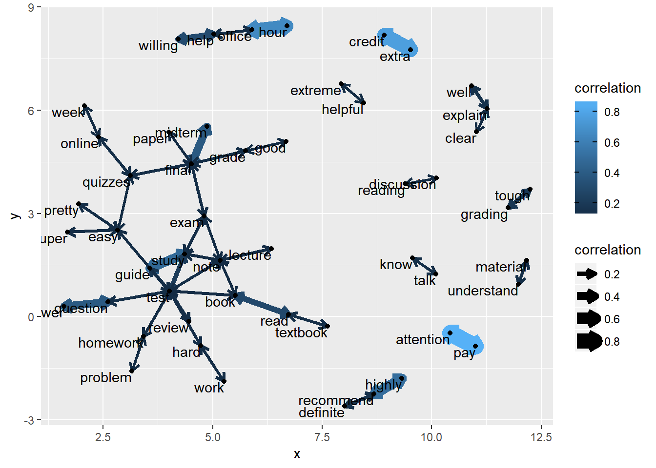
5.4 Association Rules
Pairwise count and pairwise correlation tell how a pair of words are related. One might be also interested in how more than one words are related to another word. For example, if a student mentioned words such as “easy” and “great”, he/she would be more like to recommend a professor and therefore mention the word “recommend”. This can be investigated using a method called “Market basket analysis” in which the association rules can be identified.
Market basket analysis is often used in understanding shopping behaviors. For example, through analyzing shopping transactions, we can understand which items are frequently bought together. For example, if one buys eggs, it’s highly likely she/her would buy milk. In our text mining, we can understand which words come together. Market basket analysis is conducted by mining association rules. To do so, the R package arules can be used.
The package arules has its own data format - the transaction data format. The data should have at least two columns - the transactionID and the items in that transaction. An example is given below. The data set has three transactions. In each transaction, customers bought different items.
For our data, the items would be individual words. We can convert the tidytext data to the transaction data format easily. The following code first converts the data into a document-term matrix (cast_dtm), then to a regular matrix (as.matrix), and then to the transaction data format [(]as(prof.mat, "transactions")]. Note that we also removed very sparse terms before converting data. After that, there are a total of 113 words left and the sparsity of the matrix is 94%.
prof.dtm <- prof.tm %>% count(id, word) %>% cast_dtm(id, word, n)

prof.subset <- removeSparseTerms(prof.dtm, 0.98)
prof.subset
## <<DocumentTermMatrix (documents: 38149, terms: 113)>>
## Non-/sparse entries: 258925/4051912
## Sparsity           : 94%
## Maximal term length: 13
## Weighting          : term frequency (tf)

prof.mat <- as.matrix(prof.subset)

prof.arules <- as(prof.mat, "transactions")
prof.arules
## transactions in sparse format with
##  38149 transactions (rows) and
##  113 items (columns)

inspect(prof.arules[1:10])
##      items           transactionID
## [1]  {assignment,
##       best,
##       dont,
##       like}                     1
## [2]  {best,
##       clear,
##       expect,
##       explain,
##       help,
##       homework,
##       mathematics,
##       question,
##       willing}                  2
## [3]  {clear,
##       explain,
##       homework,
##       better,
##       don't,
##       great,
##       topic,
##       understand,
##       work}                     3
## [4]  {help,
##       willing,
##       difficult,
##       extreme,
##       grade,
##       hour,
##       know,
##       material,
##       note,
##       office,
##       prepare,
##       tough}                    4
## [5]  {don't,
##       topic,
##       understand,
##       know,
##       answer,
##       talk,
##       well,
##       worst}                    5
## [6]  {mathematics,
##       work,
##       definite,
##       hard,
##       learn,
##       love,
##       semester,
##       time}                     6
## [7]  {great,
##       tough,
##       learn,
##       time,
##       easy,
##       favorite,
##       life}                     7
## [8]  {help,
##       homework,
##       work,
##       knowledgeable,
##       problem,
##       study,
##       week}                     8
## [9]  {mathematics,
##       well,
##       worst,
##       lecture}                  9
## [10] {like,
##       clear,
##       great,
##       hour,
##       office,
##       time,
##       helpful}                  10
In the data, each transaction is one comment. For example, in the first transaction/comment, there are three words - assignment, best, and like. For the second transaction/comment, there are nine words or items.
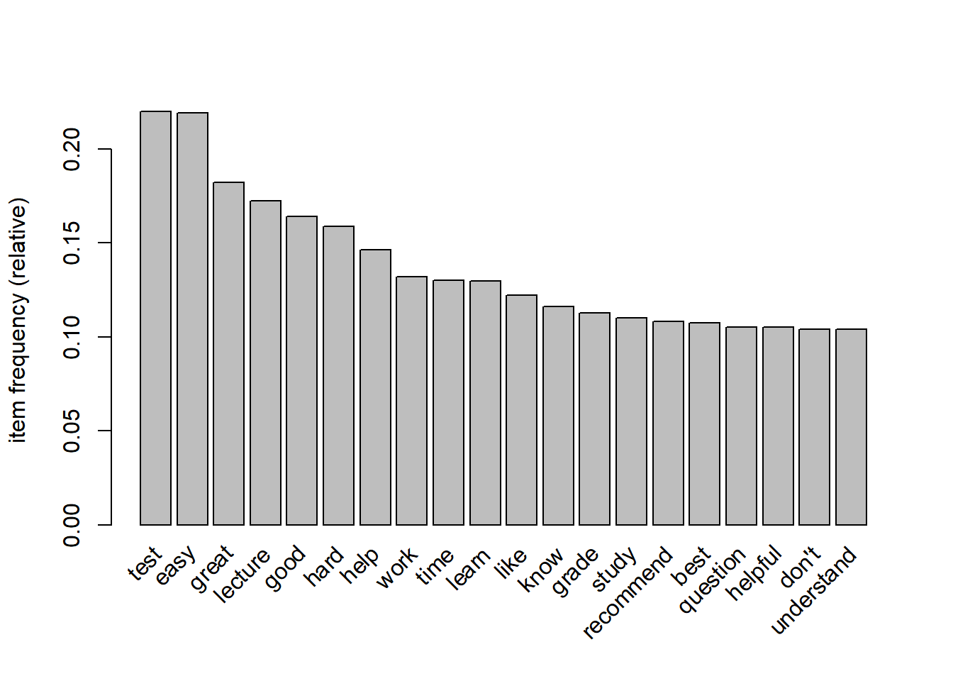
We can also check the basic information of the matrix. From the output of summary, we can see
- There are 38,149 transactions (the total number of comments) and 113 items (words).
- The most frequent items (words) are test, easy, great, lecture, and good.
- The majority of comments/transactions have around 6 words/items based on the element length distribution.
summary(prof.arules)
## transactions as itemMatrix in sparse format with
##  38149 rows (elements/itemsets/transactions) and
##  113 columns (items) and a density of 0.06006374
##
## most frequent items:
##    test    easy   great lecture    good (Other)
##    8388    8356    6946    6567    6255  222413
##
## element (itemset/transaction) length distribution:
## sizes
##    0    1    2    3    4    5    6    7    8    9   10   11   12   13   14   15
##  271 1083 2119 3096 3697 4129 4359 4134 3923 3296 2736 2031 1413  842  529  283
##   16   17   18   19   20   21   23
##  114   53   24   12    3    1    1
##
##    Min. 1st Qu.  Median    Mean 3rd Qu.    Max.
##   0.000   4.000   7.000   6.787   9.000  23.000
##
## includes extended item information - examples:
##       labels
## 1 assignment
## 2       best
## 3       dont
##
## includes extended transaction information - examples:
##   transactionID
## 1             1
## 2             2
## 3             3
5.4.1 Visualization
We can plot the top words/items in the data using the function itemFrequencyPlot.
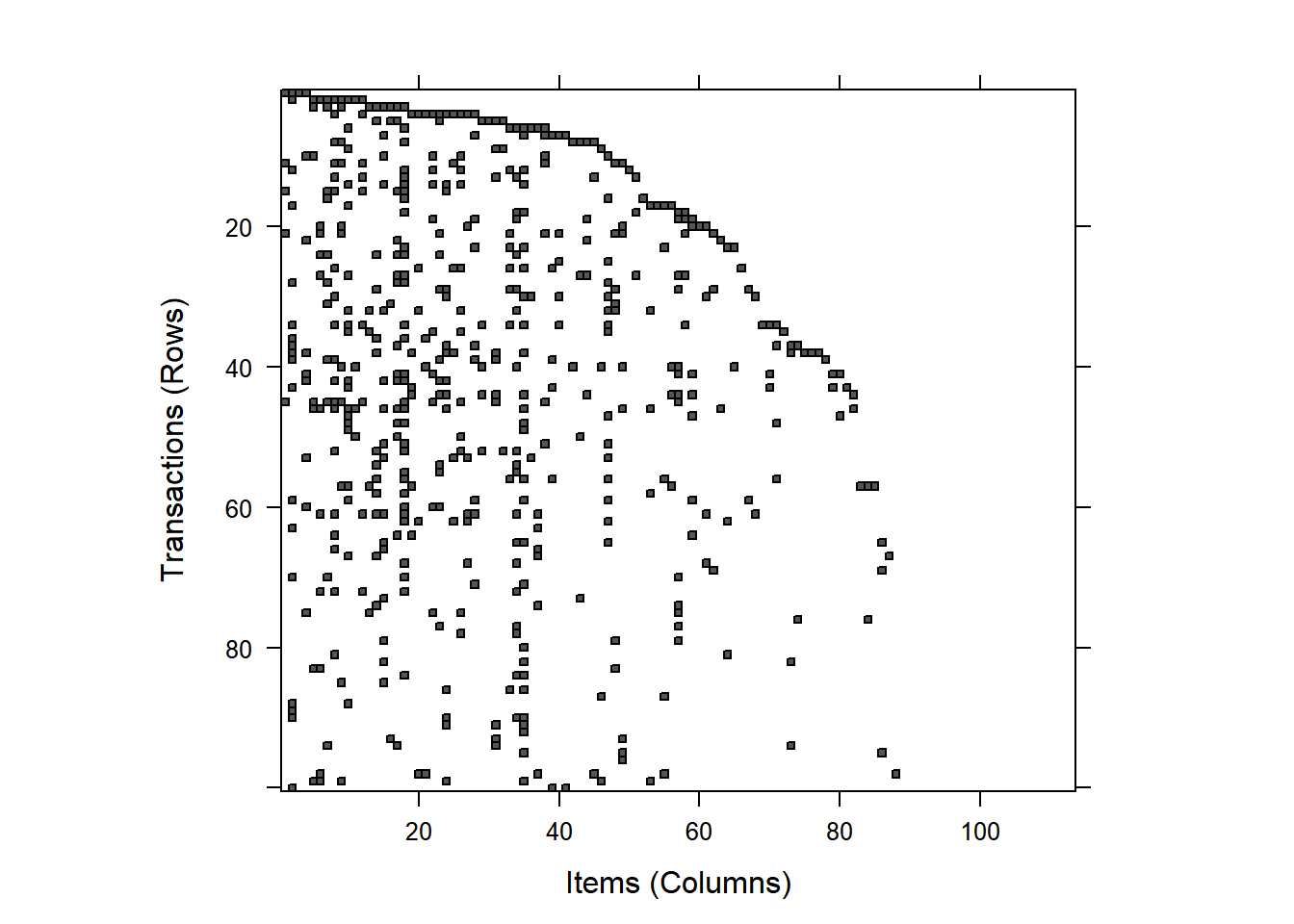
We can also plot the items for each transaction. In the plot below, a square is plotted if a transaction/comment has the item/word in the x-axis.
5.4.2 Mining rules
The R package arules has the Apriori algorithm to identify association rules in the data. A rule is to tell which word (or an item such as food) is frequently associated (bought) with another word (item). We could use the notation that Word A -> Word B to mean from Word A, we can expect Word B. THe Apriori algorithm tries to find this kind of rules.
The basic usage of the apriori function is given below.
apriori(data, parameter = list(support=0.1, confidence=0.8)
In using it, we need to decide on support and confidence. Support measures the frequency of the words, calculated as the proportion of occurrence of certain words over the total number of observations. Suppose there are two words A and B, then the support of A and B is
\[ Support (A \& B) = \frac{Number\ of\ comments\ with\ both\ A\ and\ B}{Total\ number\ of\ comments} = P\left(A \cap B\right) \]
Confidence is like a conditional probability defined as
\[ Confidence (A -> B) = \frac{Number\ of\ comments\ with\ both\ A\ and\ B}{Total\ number\ of\ times\ with\ A} = \frac{P\left(A \cap B\right)}{P\left(A\right)} \] It means given A, what is the probablity to have B in the same comment/transaction.
We can also define something called lift based on support and confidence. The higher the lift, the higher the chance of A and B occurring together.
\[ lift = \frac{Confidence (A->B)}{Support(A) \times Support(B)} = \frac{P\left(A \cap B\right)}{P\left(A\right)P\left(B\right)} \]
Oftentimes, we need to try different support and confidence to identify a set of meaningful rules. For example, when we set support to 0.005 and confidence to 0.6, we get 84 rules, with 10 rules having two words, 70 rules with 3 words and 4 rules with 4 words.
prof.rules <- apriori(prof.arules, parameter = list(support = 0.005, confidence = 0.6,
    minlen = 2))
## Apriori
##
## Parameter specification:
##  confidence minval smax arem  aval originalSupport maxtime support minlen
##         0.6    0.1    1 none FALSE            TRUE       5   0.005      2
##  maxlen target   ext
##      10  rules FALSE
##
## Algorithmic control:
##  filter tree heap memopt load sort verbose
##     0.1 TRUE TRUE  FALSE TRUE    2    TRUE
##
## Absolute minimum support count: 190
##
## set item appearances ...[0 item(s)] done [0.00s].
## set transactions ...[113 item(s), 38149 transaction(s)] done [0.01s].
## sorting and recoding items ... [113 item(s)] done [0.00s].
## creating transaction tree ... done [0.01s].
## checking subsets of size 1 2 3 4 done [0.02s].
## writing ... [84 rule(s)] done [0.00s].
## creating S4 object  ... done [0.00s].

prof.rules
## set of 84 rulessummary(prof.rules)
## set of 84 rules
##
## rule length distribution (lhs + rhs):sizes
## 2 3 4
## 10 70 4
##
## Min. 1st Qu. Median Mean 3rd Qu. Max.
## 2.000 3.000 3.000 2.929 3.000 4.000
##
## summary of quality measures:
## support confidence lift count
## Min. :0.005007 Min. :0.6065 Min. : 2.758 Min. : 191.0
## 1st Qu.:0.005806 1st Qu.:0.7859 1st Qu.: 8.592 1st Qu.: 221.5
## Median :0.006907 Median :0.8546 Median :16.930 Median : 263.5
## Mean :0.010057 Mean :0.8385 Mean :16.266 Mean : 383.7
## 3rd Qu.:0.009384 3rd Qu.:0.9112 3rd Qu.:22.041 3rd Qu.: 358.0
## Max. :0.038035 Max. :0.9784 Max. :28.373 Max. :1451.0
##
## mining info:
## data ntransactions support confidence
## prof.arules 38149 0.005 0.6All 84 rules are presented below. For the first rule, the support is about 0.025, the confidence is about 0.92 and the lift is 8.36. So it means if there is the word “guide” in the comment, then it would have the word “study” in 92% of the time in the comment. For Rule 11, if there are words “exam” and “guide”, it would have “study” in the comment 95% of the time.
inspect(prof.rules)
##      lhs                    rhs         support     confidence lift      count
## [1]  {guide}             => {study}     0.025112061 0.9202690   8.356901  958
## [2]  {midterm}           => {final}     0.019450051 0.6469050   9.681749  742
## [3]  {office}            => {hour}      0.024797505 0.8197574  19.352057  946
## [4]  {pay}               => {attention} 0.029489633 0.8978452  26.327360 1125
## [5]  {attention}         => {pay}       0.029489633 0.8647194  26.327360 1125
## [6]  {highly}            => {recommend} 0.034417678 0.8950239   8.289455 1313
## [7]  {willing}           => {help}      0.028257621 0.6857506   4.692502 1078
## [8]  {answer}            => {question}  0.031770164 0.6579805   6.254995 1212
## [9]  {credit}            => {extra}     0.038035073 0.7950685  16.289510 1451
## [10] {extra}             => {credit}    0.038035073 0.7792696  16.289510 1451
## [11] {exam,guide}        => {study}     0.005347453 0.9488372   8.616327  204
## [12] {great,guide}       => {study}     0.005006684 0.9502488   8.629145  191
## [13] {lecture,guide}     => {study}     0.006815382 0.9352518   8.492959  260
## [14] {easy,guide}        => {study}     0.008597866 0.9452450   8.583706  328
## [15] {study,guide}       => {test}      0.015229757 0.6064718   2.758261  581
## [16] {test,guide}        => {study}     0.015229757 0.9667221   8.778739  581
## [17] {easy,guide}        => {test}      0.006055205 0.6657061   3.027661  231
## [18] {easy,midterm}      => {final}     0.006946447 0.6992084  10.464536  265
## [19] {office,helpful}    => {hour}      0.006867808 0.8851351  20.895433  262
## [20] {hour,helpful}      => {office}    0.006867808 0.8424437  27.849554  262
## [21] {help,office}       => {hour}      0.009384256 0.8063063  19.034517  358
## [22] {help,hour}         => {office}    0.009384256 0.8384075  27.716124  358
## [23] {great,office}      => {hour}      0.005190175 0.9000000  21.246349  198
## [24] {great,hour}        => {office}    0.005190175 0.7388060  24.423491  198
## [25] {office,lecture}    => {hour}      0.006238696 0.8913858  21.042992  238
## [26] {office,test}       => {hour}      0.005845501 0.8168498  19.283418  223
## [27] {note,pay}          => {attention} 0.005478518 0.9675926  28.372552  209
## [28] {note,attention}    => {pay}       0.005478518 0.9207048  28.031899  209
## [29] {study,pay}         => {attention} 0.005766862 0.9523810  27.926503  220
## [30] {study,attention}   => {pay}       0.005766862 0.8835341  26.900195  220
## [31] {good,pay}          => {attention} 0.006946447 0.9397163  27.555140  265
## [32] {good,attention}    => {pay}       0.006946447 0.9201389  28.014668  265
## [33] {hard,pay}          => {attention} 0.005530944 0.8755187  25.672684  211
## [34] {hard,attention}    => {pay}       0.005530944 0.8940678  27.220904  211
## [35] {great,pay}         => {attention} 0.005845501 0.9291667  27.245795  223
## [36] {great,attention}   => {pay}       0.005845501 0.8544061  26.013360  223
## [37] {lecture,pay}       => {attention} 0.007994967 0.9413580  27.603280  305
## [38] {lecture,attention} => {pay}       0.007994967 0.8495822  25.866489  305
## [39] {easy,pay}          => {attention} 0.008859996 0.9521127  27.918637  338
## [40] {easy,attention}    => {pay}       0.008859996 0.8989362  27.369127  338
## [41] {test,pay}          => {attention} 0.009672600 0.9584416  28.104218  369
## [42] {test,attention}    => {pay}       0.009672600 0.9088670  27.671482  369
## [43] {best,highly}       => {recommend} 0.006081418 0.9280000   8.594871  232
## [44] {helpful,highly}    => {recommend} 0.005819288 0.9367089   8.675530  222
## [45] {learn,highly}      => {recommend} 0.005583370 0.9181034   8.503212  213
## [46] {help,highly}       => {recommend} 0.005688222 0.9041667   8.374133  217
## [47] {great,highly}      => {recommend} 0.009095913 0.9353100   8.662573  347
## [48] {lecture,highly}    => {recommend} 0.005373666 0.8613445   7.977527  205
## [49] {easy,highly}       => {recommend} 0.008964848 0.9243243   8.560828  342
## [50] {test,highly}       => {recommend} 0.005557157 0.8617886   7.981640  212
## [51] {willing,great}     => {help}      0.007785263 0.6734694   4.608463  297
## [52] {willing,easy}      => {help}      0.005635796 0.6803797   4.655750  215
## [53] {willing,test}      => {help}      0.006395974 0.7283582   4.984061  244
## [54] {help,answer}       => {question}  0.005190175 0.6804124   6.468241  198
## [55] {great,answer}      => {question}  0.005399879 0.7152778   6.799684  206
## [56] {answer,lecture}    => {question}  0.007182364 0.7248677   6.890849  274
## [57] {answer,easy}       => {question}  0.006631891 0.6356784   6.042984  253
## [58] {final,credit}      => {extra}     0.005059110 0.8976744  18.391719  193
## [59] {final,extra}       => {credit}    0.005059110 0.8772727  18.338125  193
## [60] {exam,credit}       => {extra}     0.007129938 0.8369231  17.147035  272
## [61] {exam,extra}        => {credit}    0.007129938 0.8242424  17.229602  272
## [62] {grade,credit}      => {extra}     0.007549346 0.8275862  16.955739  288
## [63] {grade,extra}       => {credit}    0.007549346 0.8445748  17.654621  288
## [64] {study,credit}      => {extra}     0.007549346 0.8753799  17.934946  288
## [65] {study,extra}       => {credit}    0.007549346 0.8470588  17.706546  288
## [66] {work,credit}       => {extra}     0.005137749 0.7313433  14.983896  196
## [67] {work,extra}        => {credit}    0.005137749 0.6666667  13.935708  196
## [68] {help,credit}       => {extra}     0.006422187 0.8477509  17.368876  245
## [69] {good,credit}       => {extra}     0.006736743 0.8056426  16.506155  257
## [70] {good,extra}        => {credit}    0.006736743 0.7859327  16.428793  257
## [71] {hard,credit}       => {extra}     0.006448400 0.7859425  16.102535  246
## [72] {hard,extra}        => {credit}    0.006448400 0.7500000  15.677671  246
## [73] {great,credit}      => {extra}     0.007785263 0.8510029  17.435504  297
## [74] {great,extra}       => {credit}    0.007785263 0.7857143  16.424227  297
## [75] {lecture,credit}    => {extra}     0.009567748 0.8548009  17.513320  365
## [76] {lecture,extra}     => {credit}    0.009567748 0.8057395  16.842826  365
## [77] {easy,credit}       => {extra}     0.013211355 0.8195122  16.790317  504
## [78] {easy,extra}        => {credit}    0.013211355 0.8600683  17.978490  504
## [79] {test,credit}       => {extra}     0.015334609 0.8251058  16.904920  585
## [80] {test,extra}        => {credit}    0.015334609 0.8565154  17.904222  585
## [81] {easy,study,guide}  => {test}      0.005924140 0.6890244   3.133714  226
## [82] {easy,test,guide}   => {study}     0.005924140 0.9783550   8.884376  226
## [83] {easy,test,credit}  => {extra}     0.005924140 0.8401487  17.213122  226
## [84] {easy,test,extra}   => {credit}    0.005924140 0.9076305  18.972711  226
The rules can be roughly divided into three categories: actionable, trivial, and inexplicable. Actionable means we identify something that is truly useful. Trivial means the rule does not add much to the existing knowledge. Inexplicable means it is hard to explain a rule and further investigation is needed. How to use these rules needs the input of subject experts.
##      lhs                 rhs         support     confidence lift     count
## [1]  {note,pay}       => {attention} 0.005478518 0.9675926  28.37255 209
## [2]  {test,pay}       => {attention} 0.009672600 0.9584416  28.10422 369
## [3]  {note,attention} => {pay}       0.005478518 0.9207048  28.03190 209
## [4]  {good,attention} => {pay}       0.006946447 0.9201389  28.01467 265
## [5]  {study,pay}      => {attention} 0.005766862 0.9523810  27.92650 220
## [6]  {easy,pay}       => {attention} 0.008859996 0.9521127  27.91864 338
## [7]  {hour,helpful}   => {office}    0.006867808 0.8424437  27.84955 262
## [8]  {help,hour}      => {office}    0.009384256 0.8384075  27.71612 358
## [9]  {test,attention} => {pay}       0.009672600 0.9088670  27.67148 369
## [10] {lecture,pay}    => {attention} 0.007994967 0.9413580  27.60328 305