Chapter 2 Mining Gender Information
No direct information about the gender of the professors is available in the data. However, with the narrative comments, it is possible to identify the gender of individual professors accurately. The basic idea is that in the comments, a student might use words that reflect the gender of a professor. For example, a comment from one student was given below:
Professor is by far my favorite professor I’ve had here at. He also is the tough professor I’ve ever had too, and his course are not easy. Although, his class are tough he always make time for his student and put student first in his class. You will learn a lot, and start the portfolio early! Great life advice too!
In the quote, the student mentioned “he”, “him” and “his” multiple times. This clearly indicates that the professor is male.
As another example, see the comment below from another student on a different professor. In the comment, the gender words include “she” and “her”. Therefore, we can easily assume that the professor is female.
She is one of the best voice teacher I have ever had. She may not be able to sing like she use to, but she sure know how the voice work. And she know that everyone is different so she does not use the same method with everyone. I love her!!!
The comments might not appear grammatically correct because (1) the identification information of professors were removed for privacy, and (2) some words were stemmed, e.g., “teachers” were converted to “teacher”, and “knew” to “know”.
Using just one comment can be risky. But if multiple students used the same gender words to describe a professor, the results can be very accurate. What we now need to do is to find all the gender words.
We follow the procedure below to conduct the analysis.
2.1 Step 1. Get the data into R
In the first step, we will read the comment information into R.
After taking a look at the comments, we found some common contractions were used such as he'll, he's, she'll and he's. We first replace the contractions with “he” and “she”. This can be done using the stri_replace_all_regex function of the R package stringi.
2.2 Step 2. Tokenize or break down the comments into individual words
To find the gender words in each comment, we first break down each comment into individual words using the R package tidytext. Particularly, the function unnest_tokens is used here. This creates a data set with each word on one row and combines that with other parts of the data. A new variable word is created to have an individual word on each row. Note that all the uppercase letters were also converted to lowercase ones.
2.3 Step 3. Select words with gender information
We now select the rows with gender words only. For the male, we use the words “he”, “him”, “his” and “mr”. For the female, we use the words “she”, “her” and “mrs”. There are many ways to do it, the easiest way is to use the filter function in the package `dplyr’.
library(tidyverse)  ## dplyr is a part of tidyverse collection.

male.info <- filter(prof.tm, prof.tm$word %in% c("he", "him", "his", "mr"))
male.info <- male.info[, c("id", "profid", "word")]
head(male.info)
##   id profid word
## 1  2      1   he
## 2  2      1   he
## 3  2      1   he
## 4  3      1   he
## 5  3      1   he
## 6  3      1   he
v1 %in% v2 checks whether the values in v1 appears in v2. If so, it returns TRUE and otherwise FALSE. With that, the filter function selects the rows corresponding to TRUE.
The code is equivalent to use
male.info <- prof.tm[prof.tm$word==‘him’ | prof.tm$word==‘his’ | prof.tm$word==‘he’ | prof.tm$word==‘mr’, c(‘id’,‘profid’, ‘word’)]
in the R base style.
The analysis can be streamlined using the tidy method. For example, the code below does the same work as above. The %>% is called “pipe” which is added at the end of the code to tell R to keep receiving new commands. To use the method, the easier way is to install the package collection tidyverse.
male.info <- prof.tm %>% filter(word %in% c("he", "him", "his", "mr")) %>% select(id,
    profid, word)
head(male.info)
##   id profid word
## 1  2      1   he
## 2  2      1   he
## 3  2      1   he
## 4  3      1   he
## 5  3      1   he
## 6  3      1   he
The tidyverse is a collection of R packages, including dplyr, ggplot2, purrr, readr, stringr, tibble, and tidyr, designed for data science. All packages share an underlying design philosophy, grammar, and data structures.
For a function foo that is designed with the tidyverse method such as foo(data, arg1, arg2, …), it can be streamlined using the method data %>% foo(arg1, arg2, …). The method can make the data processing involving multiple stages/steps very concise. Note that “%>%” has to be at the end of the previous line when changing lines.
2.4 Step 4. Frequency of gender words
For each professor, we can count how many times the gender words were used in the comments. A larger number of such words indicate more accurate identification of the gender of a professor. To do so, we first group the data based on the variable profid using the function group_by and then count the gender words for each professor. Note that the output is in the tiddle format, similar to data frame but with some useful features. For example, for the professor with id 1, he appears 120 times, him 35 times and his 44 times in total in all comments about the professor.
male.count <- male.info %>% group_by(profid) %>% count(word)

male.count
## # A tibble: 2,025 x 3
## # Groups:   profid [667]
##    profid word      n
##     <int> <chr> <int>
##  1      1 he      120
##  2      1 him      35
##  3      1 his      44
##  4      2 he       13
##  5      2 him       2
##  6      2 his       7
##  7      3 he      217
##  8      3 him      26
##  9      3 his     127
## 10      3 mr        1
## # ... with 2,015 more rows
A tibble can be viewed as a special form of the data frame. However, unlike a data frame, it makes the manipulation of data more anticipated. For example, when a column or row of a data frame is taken out, it is typically converted to a vector. However, in a tibble, its tibble format is reserved. More on tibble can be found on CRAN: https://cran.r-project.org/package=tibble.
2.5 Step 5. Weight the gender words
Some words can be easily misspelled but some are not. For example, for a female professor, one might use “he” in the comments. But “his” is hard to be a misspelling of “her”. Similarly for “mr” and “mrs”, they might not be as reliable as “him” or “her”. Therefore, we can assign different weights to the words. For the male words, we give weight 2 to “him” and “his”, and weight 1 to “he” and “mr”. We create a new variable called score to add to the data set.
male.score <- male.count %>% mutate(score = case_when(word == "him" ~ 2, word ==
    "his" ~ 2, word == "he" ~ 1, word == "mr" ~ 1))
male.score
## # A tibble: 2,025 x 4
## # Groups:   profid [667]
##    profid word      n score
##     <int> <chr> <int> <dbl>
##  1      1 he      120     1
##  2      1 him      35     2
##  3      1 his      44     2
##  4      2 he       13     1
##  5      2 him       2     2
##  6      2 his       7     2
##  7      3 he      217     1
##  8      3 him      26     2
##  9      3 his     127     2
## 10      3 mr        1     1
## # ... with 2,015 more rows
The function mutate is used to add the new variable score to the dataset male.count. The score is defined based on the gender variable word using the R function case_when. The new data set is saved as male.score.
2.6 Step 6. A gender index
We now multiply the frequency of the gender words with the corresponding weights to get a total score for each professor. We call it total. Here the function summarize is used to get a total score for each professor. For example, the male index for Professor 1 is 278 and 31 for Professor 2 and so on.
2.7 Step 7. Run the same for female
Using the same procedure in Step 3 to Step 6, we can get a female index for each professor. To show the advantage of “pipe”, we streamline the data manipulation as shown below.
female.total.score <- prof.tm %>% filter(word %in% c("she", "her", "hers", "mrs")) %>%
    select(id, profid, word) %>% group_by(profid) %>% count(word) %>% mutate(score = case_when(word ==
    "she" ~ 2, word == "her" ~ 2, word == "hers" ~ 2, word == "mrs" ~ 1)) %>% summarize(total = sum(score *
    n))

female.total.score
## # A tibble: 481 x 2
##    profid total
##     <int> <dbl>
##  1     10     2
##  2     15    76
##  3     21   112
##  4     26     2
##  5     27   256
##  6     28   226
##  7     29    98
##  8     34   130
##  9     39    10
## 10     42   306
## # ... with 471 more rows
Note that for Professor 10, we get a female score 2. Previously, the professor got a male score 422. Given the score difference, we might classify the professor as a male.
2.8 Step 8. Combine the information
We now combine the male and female information in one table using the full_join function based on the professor id variable. The function full_join keeps the rows of records from both data sets. Since we have the variable total in both data sets, they are renamed as total.x from the first data set and total.y from the second data set. In merging, if there is only information from one data set, a missing value is added. We also rename total.x to total.m for representing male score, and total.y to total.f for representing male score.
gender.info <- full_join(male.total.score, female.total.score, by = c("profid")) %>%
    replace(., is.na(.), 0) %>% rename(total.m = total.x, total.f = total.y)

gender.info
## # A tibble: 1,000 x 3
##    profid total.m total.f
##     <int>   <dbl>   <dbl>
##  1      1     278       0
##  2      2      31       0
##  3      3     524       0
##  4      4      74       0
##  5      5     398       0
##  6      6      58       0
##  7      7      31       0
##  8      8      53       0
##  9      9     270       0
## 10     10     452       2
## # ... with 990 more rows
2.9 Step 9. Gender classification
We now identify the gender of each professor using the total gender score. If the total male score is greater, we identify the professor as male, otherwise, female. In the perfect case, we would have the opposite gender score as 0. In the case both male and female gender scores are larger than 0, we also identify them for further investigation.
gender.info <- gender.info %>% mutate(gender = ifelse(total.m > total.f, "M", "F")) %>%
    mutate(gender.degree = ifelse(total.m > 0 & total.f > 0, 0, 1))
gender.info
## # A tibble: 1,000 x 5
##    profid total.m total.f gender gender.degree
##     <int>   <dbl>   <dbl> <chr>          <dbl>
##  1      1     278       0 M                  1
##  2      2      31       0 M                  1
##  3      3     524       0 M                  1
##  4      4      74       0 M                  1
##  5      5     398       0 M                  1
##  6      6      58       0 M                  1
##  7      7      31       0 M                  1
##  8      8      53       0 M                  1
##  9      9     270       0 M                  1
## 10     10     452       2 M                  0
## # ... with 990 more rows
The function ifelse can be considered as a short form of if (){} else {}. It has the format of ifelse(expression, true.response, false.response). For example, if the total.m is greater than total.f, we label the professor as male, otherwise female.
We now take a close look at the group of professor with both greater than 0 male and female gender scores. To do so, we plot both the male score and female score for the professors, as shown in Figure 2.1. Based on the plot, we can observe that the male scores and female scores separate very well - either male or female scores are quite large and the opposite is quite small. Therefore, in general, we can just assign the gender simply based on the larger score between a pair of male and female scores.
prof.gender <- gender.info %>% filter(gender.degree == 0)

ggplot(data = prof.gender, aes(x = 1:nrow(prof.gender))) + geom_bar(mapping = aes(y = total.m),
    stat = "identity", fill = "red") + geom_bar(mapping = aes(y = -total.f), stat = "identity",
    fill = "blue") + xlab("Professors") + ylab("score")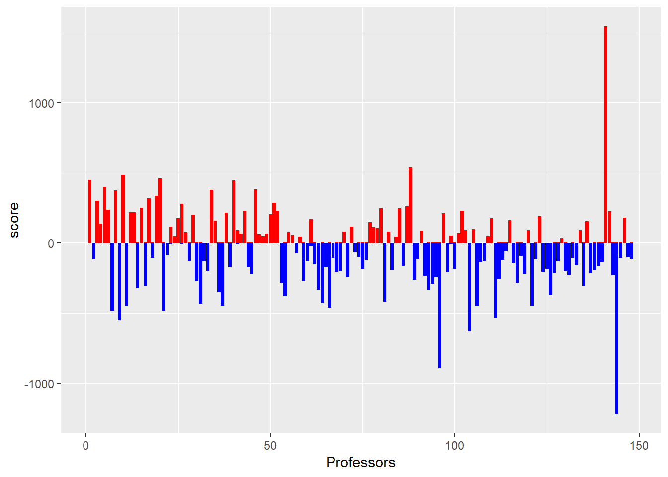
Figure 2.1: Compare the male and female score of professors
In generating the plot above, we used the R package ggplot2. To learn how to use`ggplot, start from here https://r4ds.had.co.nz/data-visualisation.html.
2.10 Save the gender information into professor data
Based on the previous steps, we can see that there are 415 female and 585 male professors in the data.
We now save the gender information into our data set. To do it, we use the R function left_join. We also remove the two variables total.m and total.f. We finally save the data into the file prof1000.stem.gender.csv for future use.
2.11 Use the gender information
The gender information can be used in many different data analyses. For example, we can compare whether the ratings for male and female professors are different. Based on the analysis, we can see that on average male professors got higher ratings than female professors.
t.test(rating ~ gender, data = prof.info)
##
##  Welch Two Sample t-test
##
## data:  rating by gender
## t = -11.547, df = 29261, p-value < 2.2e-16
## alternative hypothesis: true difference in means is not equal to 0
## 95 percent confidence interval:
##  -0.2014057 -0.1429530
## sample estimates:
## mean in group F mean in group M
##        3.671039        3.843219