Chapter 7 Topic models
We can view each comment as a combination of different themes/topics. For example, a comment may focus on the discussion of the effectiveness of teaching. However, another comment may simply talk about the personality of a professor. Some comments may have both. So the effectiveness of teaching and personality can be viewed as two topics related to teaching evaluation. Each topic is associated with certain words. For example, related to the effectiveness, words like prepared, clarity, organized and so on might be used often. Regarding the personality topic, words such as nice, open, and warm might be more often used.
The method of finding the topics and associated words is called topic modeling. Latent Dirichlet allocation (LDA) is one method for topic modeling that allows the observed words to be explained by latent topics/groups. It assumes each comment/document is a mixture of a small number of topics and each word’s presence in a comment is attributable to one of the document’s topics.
7.1 Latent Dirichlet allocation (LDA)
LDA is a popular model for topic analysis. The model can be explained in terms of the mechanism of writing a comment to evaluate teaching. In writing a comment, one might first think about from what areas to evaluate a professor. For example, a student might focus more on the organization of the lectures and the difficulty of the tests. These can be viewed as two topics. Then the student would write around the two topics by picking words related to the topics.
Suppose that there are a total of \(k\) topics. Each topic in a given document can be viewed as generating from a distribution with a different probabilities. Let \(z_{km}\) be the \(k\)th (\(k=1,\ldots, K\)) topic in the \(m\)th (\(m=1,\dots, M\)) document. \(z_{km}\) takes a value between 1 and \(K\).
\[ z_{km} \sim Multinomial(\boldsymbol{\theta}_m) \]
where \(\boldsymbol{\theta}_m=(\theta_{m1}, \theta_{m2}, \ldots, \theta_{mK})'\) is the topic probability. Note that \(\sum_{k=1}^K \theta_{mk} =1\).
Once a topic is decided, one then organizes words around it. For example, if it is about the difficulty of the test, words such as “easy” and “difficult” might be more likely used. Let \(w_{mn}, n=1,\ldots, N_d; m=1,\ldots, M\), be the \(n\)th word to be used in the \(m\)th document and \(N_d\) denoting the total number of words of the \(m\)th document. \(w_{mn}\) would take a value between 1 and \(V\) with \(V\) being the total number of unique words used in all the comments/documents. Specifically, a word is generated using
\[ w_{mn}|z_{km} \sim Multinomial(\boldsymbol{\beta}_{k}) \]
where \(\boldsymbol{\beta}_{k}=c(\beta_{k1},\beta_{k2},\ldots,\beta_{kV})'\) is the probability that a word is picked given the topic \(k\) is selected. Note that the probability is different for different words. For example, “easy” and “difficult” will have a large probability to be used in the topic regarding the test topic.
It is critical to get \(\boldsymbol{\theta}\) and \(\boldsymbol{\beta}\). The LDA assume that both are generated from a Dirichlet distribution. For topic probability, it uses
\[ \boldsymbol{\theta}_m \sim Dirichlet(\boldsymbol{\alpha}), \]
for each comment/document \(m\). For word probability, one can use
\[ \boldsymbol{\beta}_{k} \sim Dirichlet(\boldsymbol{\delta}). \]
In this case, \(\boldsymbol{\alpha}\) and \(\boldsymbol{\delta}\) are unknown parameters that can be estimated. \(\boldsymbol{\delta}_k\) has also been directly estimated as unknown parameters as in Blei et al. (2003).
7.2 Topic modeling for ratings
We use the topicmodels package for data analysis. The package uses a document-term data format (DTM). What we have now is a data matrix with each document and each word on a row from tidytext. So we first convert that into a DTM matrix using the cast_dtm function.
prof.dtm <- prof.tm %>%
        count(profid, word) %>%    ## word frequency
        cast_dtm(profid, word, n)  ## convert to dtm matrix
With it, we conduct the analysis using the following code. We first simply assume there are 2 topics and will discuss how to determine the number of topics latter.
prof.lda <- LDA(prof.dtm, k = 2)

slotNames(prof.lda)
##  [1] "alpha"           "call"            "Dim"             "control"
##  [5] "k"               "terms"           "documents"       "beta"
##  [9] "gamma"           "wordassignments" "loglikelihood"   "iter"
## [13] "logLiks"         "n"
The output of the analysis includes the following information.
- k: number of topics.
- terms: A vector containing the term names. In our case, those are different words.
- documents: A vector containing the document names, e.g., id of the professors.
- beta: logarithmized word probability for each topic, that is \(log(\boldsymbol{\beta}_{k})\).
- gamma: topic probability/proportion for each document.
- alpha: parameter of the Dirichlet distribution for topics over documents.
- wordassignments: A
simple_triplet_matrixto tell the most probable topic for each observed word in each document. This is a sparse matrix representation and can be converted to a regular matrix using the functionas.matrix.
A simple_triplet_matrix type of matrix is a representation of a sparse matrix. It can represent a regular matrix using triplets (i, j, v) of row indices i, column indices j, and values v, respectively. It can save space when the matrix is sparse.
7.2.1 Terms associated with each topic
With the output, we can first look at how each word is related to a topic. The R function terms can be directly used here to extract the most likely terms for each topic. For example, the top 10 most likely terms for the two topics are given below. From it, we can first see that the same words can be related to both topics closely such as “easy” and “grade”. The meaning of each topic can be derived based on the associated words. For example, Topic 1 here seemed to be related to the students’ perspective with words such as “work”, “learn” and “interesting”. On the other hand, Topic 2 might be more related to the professors’ activities with words such as “lecture”, “help”, “test”, and “exam”.
terms(prof.lda, 10)
##       Topic 1       Topic 2
##  [1,] "great"       "test"
##  [2,] "easy"        "lecture"
##  [3,] "work"        "easy"
##  [4,] "learn"       "hard"
##  [5,] "good"        "exam"
##  [6,] "paper"       "study"
##  [7,] "like"        "good"
##  [8,] "interesting" "question"
##  [9,] "best"        "help"
## [10,] "time"        "note"
The package tidytext provides a function tidy to re-organize the results in the tibble data format. For example, below we obtain a data set with three columns representing the topic, the term, and the associated probability with that topic. Note that for each topic, the sum of the beta values should be 1.
prof.topics <- tidy(prof.lda, matrix = "beta")
prof.topics
## # A tibble: 16,310 x 3
##    topic term            beta
##    <int> <chr>          <dbl>
##  1     1 absolute   0.00188
##  2     2 absolute   0.00110
##  3     1 accessible 0.000184
##  4     2 accessible 0.000317
##  5     1 actual     0.00356
##  6     2 actual     0.00281
##  7     1 admire     0.0000825
##  8     2 admire     0.0000141
##  9     1 advantage  0.000203
## 10     2 advantage  0.000218
## # ... with 16,300 more rows
Here we listed the top 10 most likely words associated with each topic. For example, for “easy”, it has the probability of 0.0194 within the first topic and 0.0195 within the second topic. That is to say, for all the 8815 words, the word “easy” has the probability of 0.0194 to be used within the first topic and the probability 0.0185 to be used in the second topic. Note that in the purely random sense, each of the 8815 has a probability of 1/8815=0.00011 to be used.
prof.terms <- prof.topics %>% group_by(topic) %>% top_n(10, beta) %>% ungroup() %>%
    arrange(topic, -beta)

prof.terms
## # A tibble: 20 x 3
##    topic term          beta
##    <int> <chr>        <dbl>
##  1     1 great       0.0200
##  2     1 easy        0.0199
##  3     1 work        0.0177
##  4     1 learn       0.0140
##  5     1 good        0.0124
##  6     1 paper       0.0123
##  7     1 like        0.0121
##  8     1 interesting 0.0116
##  9     1 best        0.0113
## 10     1 time        0.0112
## 11     2 test        0.0347
## 12     2 lecture     0.0240
## 13     2 easy        0.0191
## 14     2 hard        0.0172
## 15     2 exam        0.0163
## 16     2 study       0.0160
## 17     2 good        0.0148
## 18     2 question    0.0137
## 19     2 help        0.0133
## 20     2 note        0.0121
We now plot the probability and compare them.
plot.ts(log(prof.topics[prof.topics$topic == 1, "beta"]))
lines(log(prof.topics[prof.topics$topic == 2, "beta"]), col = 2)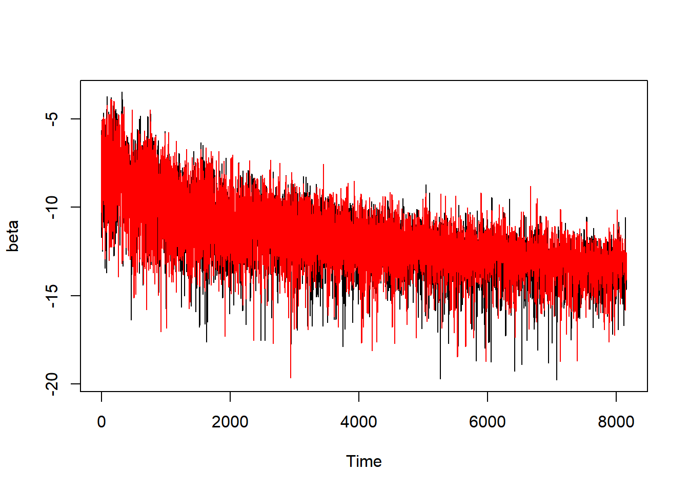
7.3 Correlated topic models
The correlated topics model (CTM; Blei and Lafferty 2007) is an extension of the LDA model where correlations between topics are allowed. Different from LDA, CTM assumes that the topic probabilities/proportions are related. Particularly, it reparametrizes the topic proportion \(\boldsymbol{\theta}_m\) as \(\eta_i = \log(\theta_i/\theta_K), i=1,\ldots, K-1\). Then for the \(\boldsymbol{\eta}_m\), it is assumed to have a multivariate normal distribution so that
\[ \boldsymbol{\eta}_m \sim N(\boldsymbol{\mu}, \boldsymbol{\Sigma}), \] where \(\boldsymbol{\mu}\) is a \(K-1\) vector and \(\boldsymbol{\Sigma}\) is a \((K-1)\times (K-1)\) matrix.
The analysis can be conducted using the CTM function. For example, suppose we have 3 topics and then the analysis can be conducted as below.
prof.ctm <- CTM(prof.dtm, k = 3, control = list(seed = 20181007))

prof.ctm
## A CTM_VEM topic model with 3 topics.

terms(prof.ctm, 10)  ## top 10 terms
##       Topic 1       Topic 2      Topic 3
##  [1,] "great"       "easy"       "test"
##  [2,] "best"        "work"       "lecture"
##  [3,] "learn"       "great"      "hard"
##  [4,] "easy"        "grade"      "exam"
##  [5,] "help"        "assignment" "good"
##  [6,] "mathematics" "test"       "question"
##  [7,] "love"        "paper"      "study"
##  [8,] "good"        "online"     "note"
##  [9,] "fun"         "time"       "material"
## [10,] "interesting" "quizzes"    "know"
topics(prof.ctm)[1:10]
##  1  2  3  4  5  6  7  8  9 10
##  1  3  3  3  2  3  1  1  1  3
We can also tidy the output of CTM for further analysis. The tidy function was originally developed for LDA. But we can trick it to work for CTM. In this case, we convert the CTM output to a LDA class using class(prof.ctm) <- "LDA_VEM".
class(prof.ctm) <- "LDA_VEM"

prof.topics <- tidy(prof.ctm, matrix = "beta")
prof.topics
## # A tibble: 24,465 x 3
##    topic term            beta
##    <int> <chr>          <dbl>
##  1     1 absolute   0.00240
##  2     2 absolute   0.000974
##  3     3 absolute   0.00121
##  4     1 accessible 0.000310
##  5     2 accessible 0.000137
##  6     3 accessible 0.000309
##  7     1 actual     0.00431
##  8     2 actual     0.00235
##  9     3 actual     0.00300
## 10     1 admire     0.0000800
## # ... with 24,455 more rows

## terms & topics
prof.terms <- prof.topics %>% group_by(topic) %>% top_n(10, beta) %>% ungroup() %>%
    arrange(topic, -beta)

prof.terms %>% print(n = 30)
## # A tibble: 30 x 3
##    topic term          beta
##    <int> <chr>        <dbl>
##  1     1 great       0.0327
##  2     1 best        0.0231
##  3     1 learn       0.0176
##  4     1 easy        0.0176
##  5     1 help        0.0161
##  6     1 mathematics 0.0151
##  7     1 love        0.0148
##  8     1 good        0.0137
##  9     1 fun         0.0131
## 10     1 interesting 0.0131
## 11     2 easy        0.0343
## 12     2 work        0.0211
## 13     2 great       0.0182
## 14     2 grade       0.0160
## 15     2 assignment  0.0160
## 16     2 test        0.0160
## 17     2 paper       0.0159
## 18     2 online      0.0139
## 19     2 time        0.0117
## 20     2 quizzes     0.0113
## 21     3 test        0.0323
## 22     3 lecture     0.0297
## 23     3 hard        0.0215
## 24     3 exam        0.0180
## 25     3 good        0.0158
## 26     3 question    0.0154
## 27     3 study       0.0142
## 28     3 note        0.0133
## 29     3 material    0.0129
## 30     3 know        0.0126
We can also visualize the topics and the strongly associated words. For example, the figure below shows the top 10 words for each topic.
prof.terms %>% mutate(term = reorder(term, beta)) %>% ggplot(aes(term, beta, fill = factor(topic))) +
    geom_col(show.legend = TRUE) + facet_wrap(~topic, scales = "free", labeller = "label_both") +
    xlab("Terms") + ylab("Topics") + coord_flip()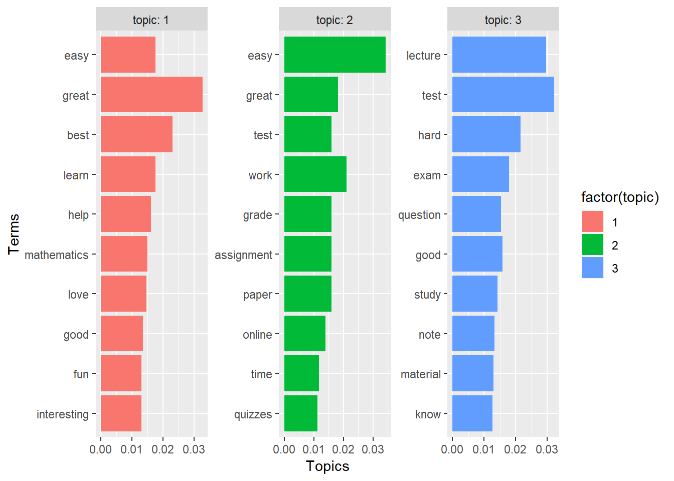
Similarly, we can look at the topics within each comment. For example, for professor 10, 25% percents of the words in the comment are from Topic 1, 71% percent from Topic 3 and only 4% from Topic 2.
7.4 Determine the number of topics
The above analysis assumes that the number of topics was known. To empirically choose the best number of topics, we can use cross-validation (CV). For example, a 5-fold cross-validation can be used. The basic idea of CV is to divide the data into 5 folds, or 5 subsets. Each time, we use 4 folds of data to fit a model and then using the left one fold of data to evaluate the model fit. This can be done for a given number of topics. Then, we can select the optimal number of topics based on a certain measure of the model fit.
In topic models, we can use a statistic – perplexity – to measure the model fit. The perplexity is the geometric mean of word likelihood. In 5-fold CV, we first estimate the model, usually called training model, for a given number of topics using 4 folds of the data and then use the left one fold of the data to calculate the perplexity. In calculating the perplexity, we set the model in LDA or CTM to be the training model and not to estimate the beta parameters.
The following code does the 5-fold CV for the number of topics ranging from 2 to 9 for LDA. Since our data have no particular order, we directly create a categorical variable folding for different folds of data. For convenience, we define a function called runonce. It takes two parameters: k for the number of topics and fold for which fold of data is used for calculating perplexity for model fit. In the function, training.dtm gets the index of data for training the model and testing.dtm for the model test. In the first LDA function, a topic model is estimated using the training data. In the second LDA function, we set the model to be training.model and
estimate.beta = FALSE. The perplexity of the test model is then obtained using the function perplexity and is returned as the output. We then run the analysis using the for loop and save all the perplexity the in the matrix res.
k.topics <- 2:9
folding <- rep(1:5, each = 200)

runonce <- function(k, fold) {
    testing.dtm <- which(folding == fold)
    training.dtm <- which(folding != fold)

    training.model <- LDA(prof.dtm[training.dtm, ], k = k)
    test.model <- LDA(prof.dtm[testing.dtm, ], model = training.model, control = list(estimate.beta = FALSE))

    perplexity(test.model)
}

res <- NULL

for (k in 2:9) {
    for (fold in 1:5) {
        res <- rbind(res, c(k, fold, runonce(k, fold)))
    }
}

res
##       [,1] [,2]      [,3]
##  [1,]    2    1 1499.9798
##  [2,]    2    2 1336.3416
##  [3,]    2    3 1228.2279
##  [4,]    2    4 1247.8692
##  [5,]    2    5  992.4989
##  [6,]    3    1 1422.6947
##  [7,]    3    2 1278.0076
##  [8,]    3    3 1205.1451
##  [9,]    3    4 1177.3957
## [10,]    3    5  938.0013
## [11,]    4    1 1408.7665
## [12,]    4    2 1269.9707
## [13,]    4    3 1191.2928
## [14,]    4    4 1163.4526
## [15,]    4    5  921.1721
## [16,]    5    1 1400.7221
## [17,]    5    2 1249.7299
## [18,]    5    3 1171.8527
## [19,]    5    4 1162.2939
## [20,]    5    5  915.9469
## [21,]    6    1 1377.8830
## [22,]    6    2 1235.1155
## [23,]    6    3 1175.1711
## [24,]    6    4 1155.6889
## [25,]    6    5  903.0834
## [26,]    7    1 1379.4431
## [27,]    7    2 1234.5547
## [28,]    7    3 1162.1048
## [29,]    7    4 1149.3635
## [30,]    7    5  899.3979
## [31,]    8    1 1376.8372
## [32,]    8    2 1237.9140
## [33,]    8    3 1175.7060
## [34,]    8    4 1148.4197
## [35,]    8    5  899.0624
## [36,]    9    1 1374.4745
## [37,]    9    2 1232.0940
## [38,]    9    3 1162.2185
## [39,]    9    4 1142.1473
## [40,]    9    5  899.9041
We now have the perplexity for each fold and can take sum or average of them. For example, the total perplexity with 2 to 9 topics is given below. We can observe that with 8 topics, we have the smallest perplexity. Therefore, we can choose k=8 topics for analysis.
total.perp <- tapply(res[, 3], res[, 1], sum)
round(total.perp)
##    2    3    4    5    6    7    8    9
## 6305 6021 5955 5901 5847 5825 5838 5811

plot(2:9, total.perp, type = "b", xlab = "Number of topics", ylab = "Perplexity")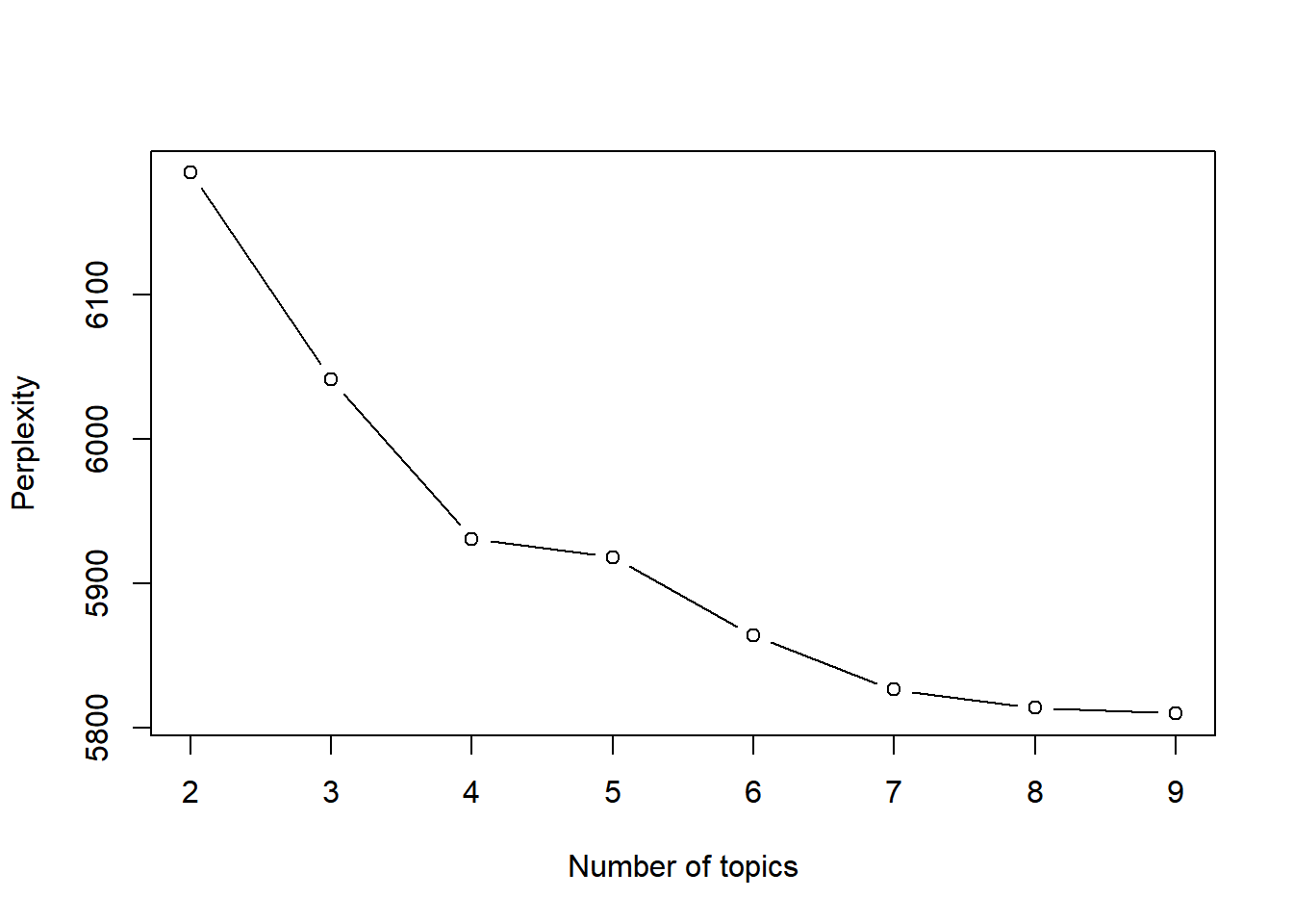
We can also compare the perplexity of each fold more closely using the plot below.
## plot the perplexity
resdata <- as.data.frame(res)
names(resdata) <- c("topics", "fold", "perplexity")
resdata$fold <- as.factor(resdata$fold)

ggplot(data = resdata, aes(x = topics, y = perplexity, group = fold, shape = fold,
    color = fold)) + geom_line() + geom_point() + scale_shape_manual(values = 1:10)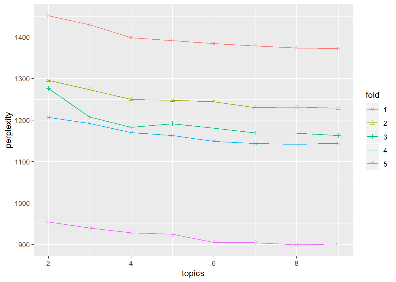
avgdata <- cbind(topics = 2:9, tapply(res[, 3], res[, 1], mean))
avgdata <- as.data.frame(avgdata)
names(avgdata) <- c("topics", "perplexity")

ggplot(data = resdata, aes(x = topics, y = perplexity, group = fold, color = fold)) +
    geom_line() + geom_point() + scale_shape_manual(values = 1:10) + geom_line() +
    geom_line(data = avgdata, aes(x = topics, y = perplexity, color = "6", size = 1.5),
        show.legend = F)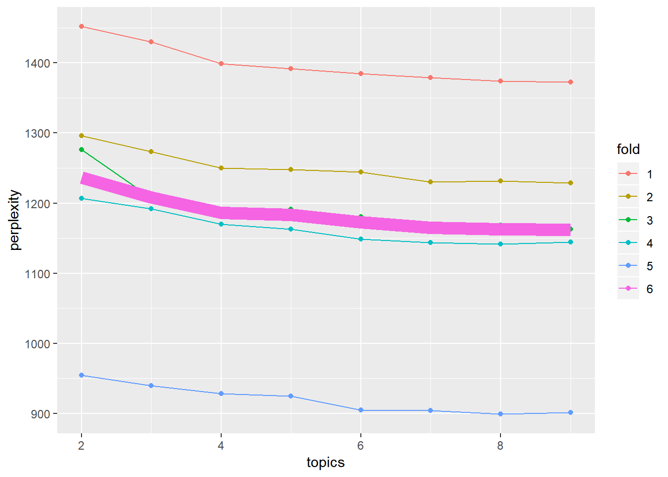
7.4.1 Analysis of teaching comments with 8 topics
Since we identify 8 topics in the comments, we can analyze the data again by setting k=8. The top 10 words related to each topic are given below. The meaning of each topic can be decided based on the top words. We also print the top 2 topics for the comments for the first 20 professors in the data. For example, for professor 1, Topic 8 and Topic 7 are most likely but for professor 2, Topic 1 and Topic 3 are more likely.
prof.lda <- LDA(prof.dtm, k = 8)

terms(prof.lda, 10)
##       Topic 1    Topic 2      Topic 3   Topic 4      Topic 5
##  [1,] "hard"     "hard"       "test"    "lecture"    "lecture"
##  [2,] "test"     "know"       "easy"    "exam"       "test"
##  [3,] "lecture"  "like"       "study"   "great"      "easy"
##  [4,] "know"     "time"       "book"    "material"   "interesting"
##  [5,] "like"     "learn"      "exam"    "easy"       "note"
##  [6,] "question" "worst"      "extra"   "question"   "good"
##  [7,] "don't"    "don't"      "quizzes" "clear"      "great"
##  [8,] "learn"    "good"       "credit"  "well"       "boring"
##  [9,] "time"     "work"       "hard"    "good"       "reading"
## [10,] "good"     "assignment" "grade"   "understand" "read"
##       Topic 6       Topic 7      Topic 8
##  [1,] "mathematics" "paper"      "great"
##  [2,] "homework"    "work"       "best"
##  [3,] "help"        "easy"       "learn"
##  [4,] "test"        "grade"      "fun"
##  [5,] "understand"  "assignment" "love"
##  [6,] "good"        "essay"      "easy"
##  [7,] "easy"        "grading"    "help"
##  [8,] "great"       "time"       "work"
##  [9,] "explain"     "reading"    "recommend"
## [10,] "problem"     "like"       "funny"
topics(prof.lda, 2)[1:2, 1:20]
##      1 2 3 4 5 6 7 8 9 10 11 12 13 14 15 16 17 18 19 20
## [1,] 6 2 5 5 7 1 8 1 1  1  3  1  2  1  7  3  2  7  6  6
## [2,] 1 6 1 4 1 2 4 5 8  5  5  8  1  3  2  1  4  8  8  5
7.5 Supervised Topic Modeling
Typically, topic models are an unsupervised learning approach to finding the structure between topics and terms as well the relationship between document and topics. In this way, we can represent the complex documents with a few important topics. However, the method focuses on the structure within the comments or documents themselves. There are times that we might want to evaluate how the comments are related to other outcomes. For example, in our teaching evaluation data, in addition to the written comments, we also have quantitative ratings of professors’ teaching quality. Then, we might want to see how the written comments are related to the quantitative teaching evaluation.
An intuitive way to do it is to first fit an unsupervised topic model such as LDA and then using the extracted topic proportion estimates of documents/comments as predictors of the outcome variables of interest. This is a two-stage approach that ignores the information between a document’s topical content and its associated outcome that could be integrated in a one-stage model. Blei and McAuliffe (2008) proposed a supervised latent Dirichlet allocation (sLDA) approach to predicting an observed univariate outcome observed and fitting a topic model simultaneously.
For sLDA, it adds a regression model above and beyond the LDA. Particularly, we model the outcome variable \(y\) as
\[ y_m = \lambda_1 \bar{z}_{1m} + \lambda_2 \bar{z}_{2m} +\ldots + \lambda_K \bar{z}_{Km} +\epsilon_m \] where \(\lambda_k\) are the regression coefficients. \(\bar{z}_{km}, k=1,\ldots, K\) are the empirical proportion of each topic in document \(m\). Particularly, it is calculated as
\[ \bar{z}_{km} = \frac{\#(z_{km}=k)}{N_m}. \] Note that since the elements of \(\bar{z}_m\) sum to 1, no intercept needs to be specified in the regression model for \(y_m\). Here, we assume that \(\epsilon_m \sim N(0, \sigma^2)\). In Blei and McAuliffe (2008), they also allow other distributions for the outcome such as binary outcomes, counts, etc., through the generalized linear model. They also showed that sLDA can outperform (1) a two-stage approach using LDA with topic proportions as predictors in a regression model and (2) LASSO using word frequencies as predictors for prediction of the outcome \(y\).
7.5.1 sLDA analysis in R
The sLDA analysis can be conducted using the R package lda.
The package requires the data to be structured as lists with words indicated by indices to an entire set of vocabularies in all the documents/comments and indicator of the word occurrences in each document. A simple example is given below to show the structure of the data. For a vector of comments or documents, we can create the desired data structure using the R function lexicalize. Note that all the words are included in the vector vocab. For each word, even the same word is used multiple times, in a document, its index (index - 1 since it starts from 0) in the vocab vector is identified as shown in the documents list.
## Generate an example.
example <- c("Professor is great and I love the class", "The class is the best I have ever taken")
corpus <- lexicalize(example, lower = TRUE)
corpus
## $documents
## $documents[[1]]
##      [,1] [,2] [,3] [,4] [,5] [,6] [,7] [,8]
## [1,]    0    1    2    3    4    5    6    7
## [2,]    1    1    1    1    1    1    1    1
##
## $documents[[2]]
##      [,1] [,2] [,3] [,4] [,5] [,6] [,7] [,8] [,9]
## [1,]    6    7    1    6    8    4    9   10   11
## [2,]    1    1    1    1    1    1    1    1    1
##
##
## $vocab
##  [1] "professor" "is"        "great"     "and"       "i"         "love"
##  [7] "the"       "class"     "best"      "have"      "ever"      "taken"
In our case, we have split the comments into individual words and removed the stopwords. Therefore, We now first put all the individual words for each professor together and then change them to the list format.
prof.nest <- prof.tm %>% group_by(profid) %>% summarise(word = paste(word, collapse = " "))

## change to lda data format
prof.lda.data <- prof.nest %>% pull(word) %>% lexicalize(lower = TRUE)
Now we are ready to fit the sLDA model. Here, we fit the model with 8 topics given our CV analysis earlier. Certainly, we can also rerun CV using sLDA. The function slda.em for the analysis requires multiple inputs.
- documents: A list whose length is equal to the number of documents. Each element of documents is an integer matrix with two rows. The first row gives the index of the terms/words. The second is simply all 1.
- K: The number of topics
- vocab: A character vector including the vocabulary words used in documents.
- params: The initial values for the regression parameters.
- annotations: The outcome variable.
params <- sample(c(-1, 1), 8, replace = TRUE)  ## starting values

# Get overall mean rating for each professor as the outcome
sy = tapply(prof1000$rating, prof1000$profid, mean)

slda_mod <- slda.em(documents = prof.lda.data$documents, K = 8, vocab = prof.lda.data$vocab,
    num.e.iterations = 100, num.m.iterations = 4, alpha = 1, eta = 0.1, params = params,
    variance = var(sy), annotations = sy, method = "sLDA")

summary(slda_mod$model)
##
## Call:
## lm(formula = annotations ~ z.bar. + 0)
##
## Residuals:
##      Min       1Q   Median       3Q      Max
## -1.45614 -0.22961  0.01114  0.23247  1.58585
##
## Coefficients:
##         Estimate Std. Error t value Pr(>|t|)
## z.bar.1  4.19586    0.08681  48.335   <2e-16 ***
## z.bar.2  0.02644    0.07175   0.369    0.713
## z.bar.3  3.57346    0.11267  31.715   <2e-16 ***
## z.bar.4  5.82846    0.09215  63.250   <2e-16 ***
## z.bar.5  3.25859    0.08060  40.428   <2e-16 ***
## z.bar.6  4.26272    0.08037  53.041   <2e-16 ***
## z.bar.7  5.64643    0.07942  71.100   <2e-16 ***
## z.bar.8  4.00679    0.06411  62.501   <2e-16 ***
## ---
## Signif. codes:  0 '***' 0.001 '**' 0.01 '*' 0.05 '.' 0.1 ' ' 1
##
## Residual standard error: 0.3627 on 992 degrees of freedom
## Multiple R-squared:  0.9911, Adjusted R-squared:  0.991
## F-statistic: 1.379e+04 on 8 and 992 DF,  p-value: < 2.2e-16
In sLDA analysis, we are primarily interested in how each topic is related to the outcome, which can be investigated based on the regression coefficient estimates. For example, all topics except for the second topic are significantly related to the numerical rating outcome.
The sLDA analysis also provides other information. For example, in the output, the object assignments includes information on how each word in a document is assigned to which topic. The object topics provides information on the number of times a word was assigned to a topic. For example, we can plot the estimated regression coefficients for each topic along with
the top five words of each topic.
# Top 5 words per topic
topics <- slda_mod$topics %>% top.topic.words(5, by.score = TRUE) %>% apply(2, paste,
    collapse = ",")

# Regression coefficients for each topic
coefs <- data.frame(coef(summary(slda_mod$model)))
coefs <- cbind(coefs, topics = factor(topics, topics[order(coefs$Estimate, coefs$Std..Error)]))
coefs <- coefs[order(coefs$Estimate), ]

coefs %>% ggplot(aes(topics, Estimate, colour = Estimate)) + geom_point() + geom_errorbar(width = 0.5,
    aes(ymin = Estimate - 1.96 * Std..Error, ymax = Estimate + 1.96 * Std..Error)) +
    coord_flip() + theme_bw()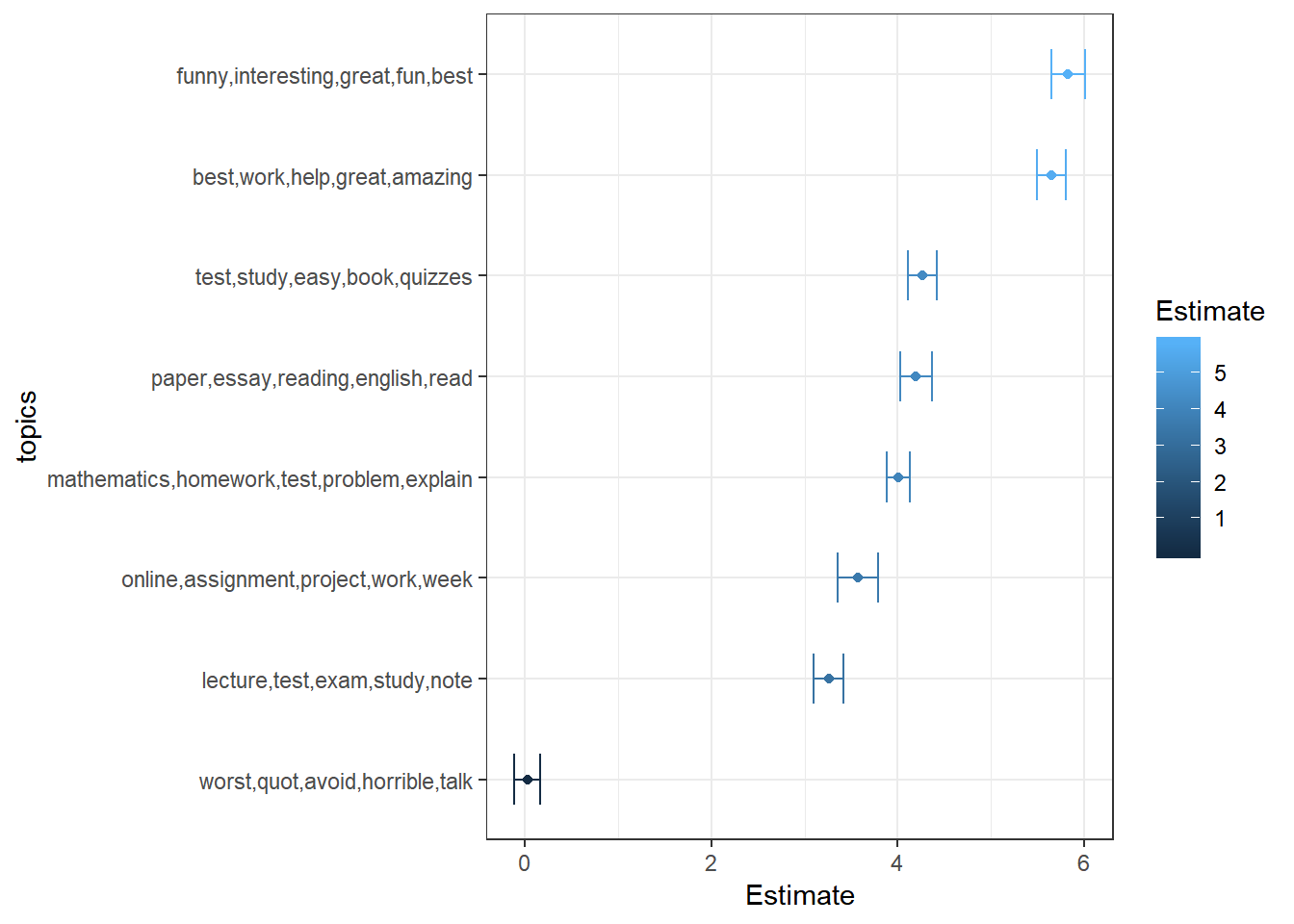
We can also get predicted ratings for the documents we’ve trained the model on (in addition to new documents with or without an observed score \(y_d\)). Here we see that our model fit seems to be reasonable.
yhat <- slda.predict(prof.lda.data$documents, slda_mod$topics, slda_mod$model,
                     alpha = 1.0, eta = 0.1)

qplot(yhat,
      xlab = "Predicted Overall Rating",
      ylab = "Density", fill = 1,
      alpha=I(0.5), geom = "density") +
      theme_bw() +
      theme(legend.position = "none") +
      geom_density(aes(sy), fill = 2, alpha = I(0.5))
With the predicted valus, we can also calculate the predicted \(R^2\) as a metric of model fit,
\[R^2 = \frac{Var[\hat{y}]}{Var[Y]} = 79.9\%.\]
7.2.2 comments associated with each topic
The R function
topicscan be directly used here to extract the most likely topics for each document/comment. For example, for the first 10 professors’ comments, the first one is most likely formed by topic 2 and the second by topic 1 and so on.We can also tidy the output to get more information. The following data table shows the proportion of words from each topic. For example, for document 1, 47.1% of words are from topic 1 and for document 2, 48.5% of words are from topic 1.
Furthermore, for a given document/comment, we can see the contribution of each topic. For example, for the 10th professor, 57% of words for his/her comments were related to topic 1 and 43% related to topic 2.