Chapter 8 Sentiment Analysis
Each word can be assigned an emotion or sentiment such as positive or negative or other categories such as happy, joy, fear, etc. The sentiment of each word can be best identified for a particular problem. For example, when studying positive and negative affects, one can ask people to identify whether a word shows positive or negative meanings.
8.1 Word sentiment
In the literature, there are three sentiment dictionaries or lexicons with identified word meaning that are widely used - AFINN, nrc, and bing.
8.1.1 AFINN
The AFINN lexicon assigns words with a score between -5 and 5, with negative scores indicating negative sentiment and positive scores indicating positive sentiment. AFINN includes 2,476 words in total. For a complete list with the scores see AFINN word list. Some example words and their associated scores are given below.
get_sentiments("afinn")
## # A tibble: 2,476 x 2
##    word       score
##    <chr>      <int>
##  1 abandon       -2
##  2 abandoned     -2
##  3 abandons      -2
##  4 abducted      -2
##  5 abduction     -2
##  6 abductions    -2
##  7 abhor         -3
##  8 abhorred      -3
##  9 abhorrent     -3
## 10 abhors        -3
## # ... with 2,466 more rows

get_sentiments("afinn") %>% filter(score == 5)
## # A tibble: 5 x 2
##   word         score
##   <chr>        <int>
## 1 breathtaking     5
## 2 hurrah           5
## 3 outstanding      5
## 4 superb           5
## 5 thrilled         5

get_sentiments("afinn") %>% filter(score == -5)
## # A tibble: 16 x 2
##    word           score
##    <chr>          <int>
##  1 bastard           -5
##  2 bastards          -5
##  3 bitch             -5
##  4 bitches           -5
##  5 cock              -5
##  6 cocksucker        -5
##  7 cocksuckers       -5
##  8 cunt              -5
##  9 motherfucker      -5
## 10 motherfucking     -5
## 11 niggas            -5
## 12 nigger            -5
## 13 prick             -5
## 14 slut              -5
## 15 son-of-a-bitch    -5
## 16 twat              -5
8.1.2 nrc
The nrc lexicon categorizes words into positive or negative sentiments as well as 8 different emotions including anger, anticipation, disgust, fear, joy, sadness, surprise, and trust. For a complete list with the categories see nrc word list. In total, 6,468 words were rated.
get_sentiments("nrc")
## # A tibble: 13,901 x 2
##    word        sentiment
##    <chr>       <chr>
##  1 abacus      trust
##  2 abandon     fear
##  3 abandon     negative
##  4 abandon     sadness
##  5 abandoned   anger
##  6 abandoned   fear
##  7 abandoned   negative
##  8 abandoned   sadness
##  9 abandonment anger
## 10 abandonment fear
## # ... with 13,891 more rows
8.1.3 bing
The bing lexicon categorizes words in a binary fashion into positive and negative categories. For a complete list with the categories see bing word list. In total, 6,788 words are rated.
get_sentiments("bing")
## # A tibble: 6,788 x 2
##    word        sentiment
##    <chr>       <chr>
##  1 2-faced     negative
##  2 2-faces     negative
##  3 a+          positive
##  4 abnormal    negative
##  5 abolish     negative
##  6 abominable  negative
##  7 abominably  negative
##  8 abominate   negative
##  9 abomination negative
## 10 abort       negative
## # ... with 6,778 more rows
8.2 Basic sentiment analysis
For each comment, we can calculate its overall sentiment. To quantify the emotion or sentiment of a comment, we score it based on individual words. We first use the afinn lexicon for sentiment analysis. This can be done using the code below. Note that we add a new column called score to the dataset. For the word “best”, its score is 3, but for the word “odd” its score is -2.
rating.sentiment <- prof.tm %>% inner_join(get_sentiments("afinn"))

rating.sentiment[1:10, c("word", "score")]
##         word score
## 1       best     3
## 2       like     2
## 3       best     3
## 4       help     2
## 5      clear     1
## 6      great     3
## 7      clear     1
## 8        odd    -2
## 9     better     2
## 10 respected     2
We can now calculate the overall sentiment of a comment based on the scores of all the individual words. Basically, we add all the scores of the words for a comment together. For future analysis, we also get the numerical rating of teaching and the difficulty of the class. From the output, we can see that the overall sentiment of the first comment is 5 and for the fifth comment is -10.
prof.tm.sentiment <- rating.sentiment %>% group_by(id) %>% summarise(rating = mean(rating),
    difficulty = mean(difficulty), sentiment = sum(score))

prof.tm.sentiment
## # A tibble: 37,397 x 4
##       id rating difficulty sentiment
##    <int>  <dbl>      <dbl>     <int>
##  1     1      5          3         5
##  2     2      5          4         6
##  3     3      4          5         4
##  4     4      3          5         5
##  5     5      1          5       -10
##  6     6      5          5         4
##  7     7      5          5         6
##  8     8      2          4         0
##  9     9      3          5         1
## 10    10      3          5         2
## # ... with 37,387 more rows
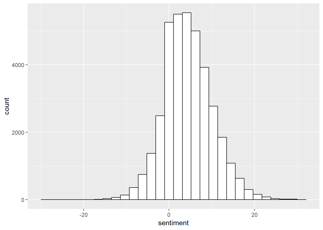
The histogram of the sentiment scores of all the comments is shown below. The distribution seems to be symmetric but with long tails.
prof.tm.sentiment %>% ggplot(aes(sentiment)) + geom_histogram(color = "black", fill = "white",
    bins = 30)
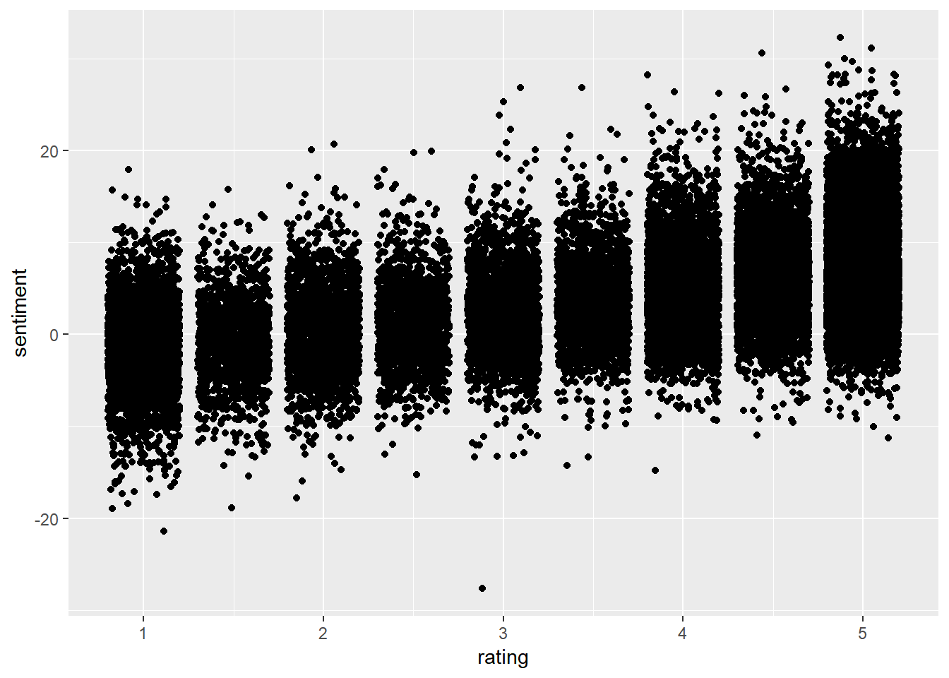
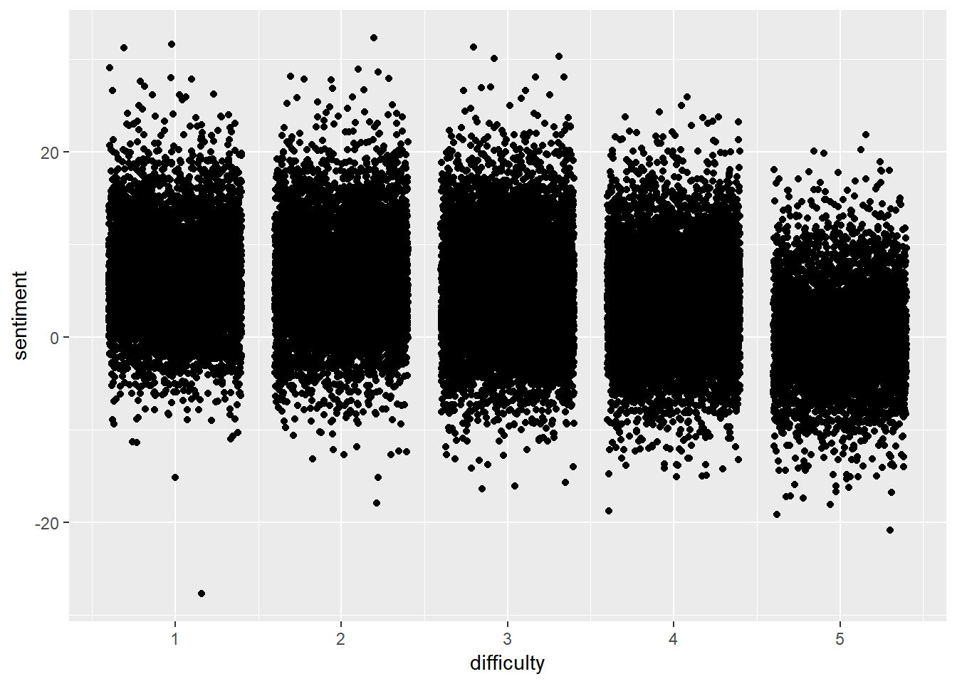
We then look at the relationship between the rating and the sentiment of the comment using Pearson correlation, which is 0.56, a quite large correlation. The correlation between the sentiment and the difficulty is negative.
cor(prof.tm.sentiment[, 2:4])
##                rating difficulty  sentiment
## rating      1.0000000 -0.4768910  0.5635187
## difficulty -0.4768910  1.0000000 -0.3164134
## sentiment   0.5635187 -0.3164134  1.0000000

prof.tm.sentiment %>% ggplot(aes(x = rating, y = sentiment)) + geom_jitter()

geom_jitter is a convenient shortcut for geom_point(position = “jitter”). It adds a small amount of random variation to the location of each point, and is a useful way of handling overplotting caused by discreteness in smaller datasets.
8.3 2-gram sentiment analysis
The sentiment analysis was based on individual words. In a comment, there are often words such “not” and “don’t” that can give the single word opposite meaning. For example, “good” is, in general, a positive word but “not good” is negative. Therefore, we would need to identify the negative meaning of phrases such as not good, not useful, etc. This can be done by dividing the two words. For the first word, we can find negative words such as not, no, never, etc. Then, we can score the second word as in the previous sentiment analysis. After that, we change the direction of the sentiment for those with proceeding negative words.
The following code first uses 2grams to divide the comments into consecutive two words. After that, we break down the two words into two columns - word1 and word2. We then score word2 using the sentiment word list.
prof.tm <- unnest_tokens(prof1000, word, comments, token = "ngrams", n = 2)

prof.separated <- prof.tm %>% separate(word, c("word1", "word2"), sep = " ")

rating.sentiment <- prof.separated %>% inner_join(get_sentiments("afinn"), by = c(word2 = "word"))
We now identify a list of words that would flip the sentiment of the words following them.
negativeword <- c("no", "not", "never", "dont", "don't", "cannot", "can't", "won't",
    "wouldn't", "shouldn't", "aren't", "isn't", "wasn't", "weren't", "haven't", "hasn't",
    "hadn't", "doesn't", "didn't", "mightn't", "mustn't")
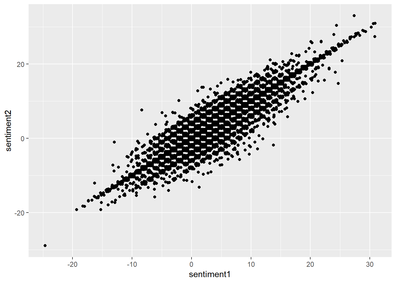
We now create a new score2 variable that takes into account the negative words. The code for the analysis is given below. Note that we increased the correlation from 0.563 to 0.575. The increase is not dramatic. Actually, the two sentiment scores are highly correlated with a correlation of 0.96.
rating.sentiment <- rating.sentiment %>% mutate(score1 = score, score2 = ifelse(word1 %in%
    negativeword, -score, score))

prof.tm.sentiment <- rating.sentiment %>% group_by(id) %>% summarise(rating = mean(rating),
    easy = mean(difficulty), sentiment1 = sum(score1), sentiment2 = sum(score2))

cor(prof.tm.sentiment[, 2:5])
##                rating       easy sentiment1 sentiment2
## rating      1.0000000 -0.4771256  0.5331909  0.5747061
## easy       -0.4771256  1.0000000 -0.2962231 -0.3261040
## sentiment1  0.5331909 -0.2962231  1.0000000  0.9595544
## sentiment2  0.5747061 -0.3261040  0.9595544  1.0000000

prof.tm.sentiment %>% ggplot(aes(x = sentiment1, y = sentiment2)) + geom_jitter()