Chapter 8 Big data
It is well accepted that the meaning of big data is context specific and evolving over time (e.g., De Mauro et al., 2016; Fox, 2018). In his 1998 talk at the USENIX conference, John Mashey discussed the problems and future of big data (Mashey, 1998). At that time, a desktop with 256MB of random-access memory (RAM; also called physical memory or just memory) and 16GB (1GB=1000MB or 1024MB) of hard drive (or disk drive, or just disk) was considered to be a “monster” machine costing more than $3,000. In July 2018, a laptop with 8GB of RAM and 1000GB of hard drive may cost less than $400 (e.g., a Lenovo A12-9720P). Clearly, a “big” data set in 1998 could be a “small” data set in 2018. Thus, big data should not be defined simply by the size of the data but should be considered as “data sets that are so big and complex that traditional data-processing application software is inadequate to deal with them” (Wikipedia).
R conducts all the operations directly in RAM, and thus is not well-suited for working with data larger than 10-20% of the computer RAM (R Manual). The usage of memory in R can increase dramatically when conducting calculations.
8.1 Memory management in R
When R starts, it sets up a workspace. The size of the workspace changes according to the data and operations. Anything in the workspace can be viewed as an R object, being a number, vector or matrix. The objects can be fixed-sized or variable sized. In R, these are called Ncells and Vcells.
For example, the function gc() can tell us the memory usage information. The last column of Vcells shows the maximum space/memory used.
gc()
##              used    (Mb) gc trigger    (Mb)   max used    (Mb)
## Ncells   12605253   673.2   31275138  1670.3   31275138  1670.3
## Vcells 2469717191 18842.5 3842207646 29313.8 3842207009 29313.8

gc(reset=TRUE)
##              used    (Mb) gc trigger    (Mb)   max used    (Mb)
## Ncells   12604823   673.2   31275138  1670.3   12604823   673.2
## Vcells 2469716482 18842.5 3842207646 29313.8 2469716482 18842.5
The R function object.size can be used to calculate the size of an R object.
a <- rnorm(10000)
object.size(a)
## 80048 bytes

format(object.size(a), 'Kb')
## [1] "78.2 Kb"
format(object.size(a), 'Mb')
## [1] "0.1 Mb"
We can log the use of memory in R, too, which is called memory profiling. This can be done using the R package profmem.
library(profmem)

profmem(
  {
    a <- array(rnorm(1000), dim=c(100,10))
    b <- array(rnorm(1000), dim=c(100,10))
    a + b
  }
)
## Rprofmem memory profiling of:
## {
##     a <- array(rnorm(1000), dim = c(100, 10))
##     b <- array(rnorm(1000), dim = c(100, 10))
##     a + b
## }
##
## Memory allocations:
##        what bytes              calls
## 1     alloc  8048 array() -> rnorm()
## 2     alloc  2552 array() -> rnorm()
## 3     alloc  8048            array()
## 4     alloc  8048 array() -> rnorm()
## 5     alloc  2552 array() -> rnorm()
## 6     alloc  8048            array()
## 7     alloc  8048         <internal>
## total       45344
8.2 Investigate the memory usage of R
We first define a function to output the size of an R object.
msize <- function(x){
  format(object.size(x), units = "auto")
}
Now, let’s generate a data set with 1,000 subjects and 100 variables. The data set takes about 781.5 Kb memory.
N <- 1000
P <- 100
y <- array(rnorm(N*P), dim=c(N,P))
msize(y)
## [1] "781.5 Kb"
If we are interested in the variance and covariance matrix of the data, we will have a 100 by 100 matrix that takes about 78.3 Kb of memory.
cov.y <- cov(y)
msize(cov.y)
## [1] "78.3 Kb"
The covariance matrix is symmetric and there are 100*(100+1)/2 = 5,050 estimated values. In statistical inference, we may need to get the covariance matrix of these 5,050 values. Then this will result in a matrix of the size 5,050 by 5,050. The matrix is related to the outer product of the sample covariance matrix. Note that such a matrix already takes 762.9 Mb of memory.
cov.cov.y <- cov.y %o% cov.y
msize(cov.cov.y)
## [1] "762.9 Mb"
Now consider another example. In a study, I have data on 45 variables from more than 9 million participants. Since I cannot share the data, I generate a data set instead of using the following code.
x <- array(rnorm(9300000*44), dim=c(9300000, 44))
y <- x%*%c(0.8, 0.5, rep(0, 42))
y <- y + rnorm(9300000)

dset <- cbind(y, x)

write.table(round(dset,3), "bigdata1.txt", quote='', col.names=F, row.names=F)
The data file itself takes 2.49Gb disk space on the hard drive. It took 255.64 seconds to read the whole data set into R and the R matrix takes 3.1 Gb of memory.
system.time(bigdata <- read.table('D:/data/bigdata1.txt'))
##    user  system elapsed
##  120.02    4.47  124.86
names(bigdata) <- c('y', paste0('x', 1:44))
msize(bigdata)
## [1] "3.1 Gb"
Since a file can be very large and can be difficult to read all together or even open, it is useful to take a look at the first part of the data. This can be done using R function readLines which can read data line by line.
# read the first 3 lines of the file
readLines('D:/data/bigdata1.txt', n=10)
##  [1] "0.078 0.758 -0.694 -0.947 -2.581 -0.149 -0.2 1.964 0.326 0.992 0.881 1.62 2.207 0.372 0.38 1.351 1.971 0.474 0.03 0.959 -0.675 -0.024 -0.102 -1.448 -1.158 0.01 -1.184 -0.572 0.52 -0.608 -0.547 0.598 -0.567 1.471 -1.067 -0.452 0.916 0.379 -0.943 -1.19 -0.086 -1.576 -0.6 1.452 0.189"
##  [2] "2.698 2.123 0.131 -0.918 1.051 -0.701 -0.302 1.344 0.328 -0.49 -0.837 -0.658 0.95 0.123 1.191 -0.272 0.086 1.179 0.707 -0.891 -1.135 1.082 -0.332 -0.474 -0.974 -1.049 0.685 -0.203 -1.67 -0.783 -1.205 -1.23 0.5 -0.522 -0.007 1.652 0.104 -0.489 -0.823 -0.013 0.324 0.257 1.557 -0.645 0.619"
##  [3] "-0.504 0.357 -1.48 -0.426 -1.107 1.407 -0.847 1.979 0.23 0.673 -0.601 0.242 1.543 0.206 0.241 -0.095 0.432 -0.243 0.265 2.195 2.175 -0.394 1.12 -0.834 2.391 2.097 -1.66 1.927 -0.349 -0.882 -0.1 0.382 -1.084 0.136 0.331 0.413 0.103 -0.609 0.964 1.03 -0.007 0.879 -0.585 -0.194 0.485"
##  [4] "-0.886 -2.327 -0.48 1.08 1.882 -0.323 -0.913 -0.307 0.594 0.397 -0.522 -0.312 -3.415 -0.882 0.653 1.569 -1.102 0.391 0.364 -0.396 0.822 1.373 -1.385 1.044 1.144 -3.073 1.086 -0.516 0.31 -0.425 2.31 0.366 -0.739 0.434 -1.526 -0.196 -0.982 -1.372 -2.034 -0.48 0.102 -2.111 0.036 1.363 0.696"
##  [5] "2.454 0.216 1.52 0.504 -0.471 -0.04 -0.333 0.446 0.105 0.041 -1.003 -0.684 -0.877 1.505 -1.629 -0.786 0.789 -0.139 0.798 1.873 -0.223 -1.333 0.846 -0.604 -2.525 0.082 -0.675 -0.807 -0.939 -0.258 -0.024 0.141 -0.008 0.897 0.661 -0.503 1.255 -1.544 1.516 -0.702 0.281 -0.85 0.171 -0.182 -1.084"
##  [6] "1.52 0.877 0.769 -0.747 -0.044 -2.161 -0.106 -0.936 0.631 2.725 -0.075 1.933 0.722 0.68 -1.868 -2.974 -0.279 -1.296 1.544 0.992 0.385 0.222 0.13 0.757 0.011 0.187 -1.113 -1.004 0.104 0.542 0.393 -1.25 -0.277 0.155 0.188 -0.271 0.623 0.226 0.786 2.519 -0.126 -0.134 2.008 -0.168 -0.428"
##  [7] "-1.585 -1.163 0.143 0.218 -0.964 -0.767 1.322 0.884 1.729 0.266 -0.149 -2.203 -0.095 0.223 -0.822 1.915 -2.257 0.972 1.799 1.462 0.228 0.828 -1.316 0.17 -1.131 0.917 0.81 1.576 -1.008 -1.492 1.514 -0.711 -0.591 1.267 -0.917 -0.729 0.891 -0.476 -1.021 0.868 1.45 1.482 1.648 -0.551 -2.253"
##  [8] "-1.961 -2.201 -0.469 0.621 -1.164 0.163 -1.664 -2.007 -0.743 -0.755 1.337 0.132 0.96 0.588 -0.787 1.223 2.55 0.472 -0.299 1.223 0.142 -1.267 2.004 0.144 0.819 1.792 -0.647 -0.887 0.399 -0.31 0.828 0.339 0.036 -0.77 -0.809 -1.145 0.238 -1.091 0.844 -0.105 -0.159 -1.74 0.029 0.462 2.003"
##  [9] "3.825 1.77 2.539 -2.003 0.648 -2.177 1.254 -0.297 0.919 -0.323 -1.848 0.515 0.009 0.726 -0.912 -2.591 -0.341 -1.609 1.289 0.66 1.33 0.297 0.057 0.489 0.589 -0.228 -0.59 0.763 -0.904 -1.477 2.413 -0.822 -0.695 -0.266 -0.737 -0.036 -0.67 1.591 -1.311 -0.188 -0.22 -0.416 -1.697 -0.433 -1.031"
## [10] "0.656 1.849 -2.221 -0.062 2.957 1.688 -1.318 1.223 0.747 -1.027 1.256 -0.16 0.842 1.61 -0.244 -0.435 -0.548 -0.352 0.885 0.046 1.796 -1.782 1.647 0.67 0.746 0.64 2.618 -0.037 0.506 -2.157 0.307 0.543 0.379 -0.31 -1.676 -0.052 -2.249 1.828 1.473 -0.445 -1.338 -0.812 0.493 1.182 0.374"
For the data, we can fit a regression model.
gc(reset = TRUE)
##              used    (Mb) gc trigger    (Mb)   max used    (Mb)
## Ncells   12604862   673.2   31275138  1670.3   12604862   673.2
## Vcells 2469819313 18843.3 3842207646 29313.8 2469819313 18843.3
system.time(lm.model <- lm(y ~ ., data=bigdata))
##    user  system elapsed
##   31.28    5.81   37.10
gc()
##              used    (Mb) gc trigger    (Mb)   max used    (Mb)
## Ncells    3305513   176.6   25020110  1336.3   12622298   674.2
## Vcells 2441919986 18630.4 4610729175 35177.1 3841579592 29309.0

summary(lm.model)
##
## Call:
## lm(formula = y ~ ., data = bigdata)
##
## Residuals:
##     Min      1Q  Median      3Q     Max
## -5.5016 -0.6746  0.0000  0.6746  4.9972
##
## Coefficients:
##               Estimate Std. Error  t value Pr(>|t|)
## (Intercept) -2.661e-04  3.278e-04   -0.812  0.41695
## x1           8.003e-01  3.279e-04 2440.811  < 2e-16 ***
## x2           4.999e-01  3.278e-04 1525.104  < 2e-16 ***
## x3          -4.739e-04  3.279e-04   -1.445  0.14838
## x4          -3.020e-04  3.279e-04   -0.921  0.35701
## x5          -4.545e-04  3.278e-04   -1.387  0.16558
## x6          -1.948e-04  3.278e-04   -0.594  0.55242
## x7          -2.488e-04  3.278e-04   -0.759  0.44785
## x8           3.362e-04  3.278e-04    1.026  0.30506
## x9           4.538e-04  3.278e-04    1.384  0.16632
## x10         -5.771e-04  3.278e-04   -1.760  0.07833 .
## x11         -1.368e-04  3.278e-04   -0.417  0.67647
## x12         -1.840e-04  3.279e-04   -0.561  0.57464
## x13          3.161e-04  3.278e-04    0.964  0.33488
## x14         -2.598e-04  3.277e-04   -0.793  0.42797
## x15         -3.631e-04  3.279e-04   -1.107  0.26811
## x16          1.382e-04  3.278e-04    0.422  0.67337
## x17          2.026e-04  3.279e-04    0.618  0.53661
## x18          5.563e-05  3.278e-04    0.170  0.86526
## x19          3.374e-05  3.279e-04    0.103  0.91805
## x20         -9.403e-04  3.279e-04   -2.867  0.00414 **
## x21         -1.072e-04  3.277e-04   -0.327  0.74359
## x22          5.049e-04  3.279e-04    1.540  0.12365
## x23         -2.200e-04  3.278e-04   -0.671  0.50212
## x24          4.885e-04  3.278e-04    1.490  0.13610
## x25         -1.226e-04  3.278e-04   -0.374  0.70846
## x26         -4.829e-05  3.278e-04   -0.147  0.88287
## x27         -5.505e-04  3.278e-04   -1.680  0.09302 .
## x28          7.486e-05  3.279e-04    0.228  0.81940
## x29         -6.634e-04  3.279e-04   -2.023  0.04308 *
## x30         -1.978e-04  3.278e-04   -0.604  0.54617
## x31          7.914e-04  3.278e-04    2.414  0.01576 *
## x32         -1.750e-04  3.279e-04   -0.534  0.59352
## x33          9.689e-05  3.279e-04    0.295  0.76764
## x34         -1.413e-04  3.278e-04   -0.431  0.66649
## x35          5.080e-04  3.278e-04    1.550  0.12123
## x36         -2.867e-04  3.280e-04   -0.874  0.38215
## x37         -2.032e-04  3.278e-04   -0.620  0.53528
## x38         -1.623e-04  3.277e-04   -0.495  0.62039
## x39          2.997e-04  3.278e-04    0.914  0.36056
## x40          3.403e-06  3.278e-04    0.010  0.99172
## x41          2.188e-04  3.279e-04    0.667  0.50448
## x42          1.713e-04  3.279e-04    0.522  0.60140
## x43          8.022e-05  3.279e-04    0.245  0.80676
## x44          7.804e-04  3.278e-04    2.381  0.01728 *
## ---
## Signif. codes:  0 '***' 0.001 '**' 0.01 '*' 0.05 '.' 0.1 ' ' 1
##
## Residual standard error: 0.9998 on 9299955 degrees of freedom
## Multiple R-squared:  0.471,  Adjusted R-squared:  0.471
## F-statistic: 1.882e+05 on 44 and 9299955 DF,  p-value: < 2.2e-16
The whole analysis took about 33 seconds. It increased the memory usage from 10.3Gb to 23.38Gb, which means the analysis would use about 13Gb of memory. The model results, lm.model, use about 8.2Gb of memory. On computers without large enough memory, errors would occur.
msize(lm.model)
## [1] "8.2 Gb"
8.3 Ways for handling big data
Many different ways can be used to handle big data. For example, one can use more powerful computers with more memory and more powerful CPUs to analyze big data. One can also use better algorithms that require less computer memory. Here we consider the following methods: (1) use sparse matrix, (2) use file-backed memory management, and (3) use a divide-and-conquer algorithm.
8.3.1 Use of the sparse matrix
In general, a matrix with many zeros is called a sparse matrix and, otherwise, a dense matrix. For example, see the matrix below. It contains only 9 nonzero elements, with 26 zero elements. Its sparsity is 26/35 = 74%, and its density is 9/35 = 26%.
mat1 <- array(c(11,0,0,0,0, 22,33,0,0,0, 0,44,55,0,0,
                 0,0,66,0,0, 0,0,77,0,0, 0,0,0,88,0,
                 0,0,0,0,99), dim=c(5,7))

mat1
##      [,1] [,2] [,3] [,4] [,5] [,6] [,7]
## [1,]   11   22    0    0    0    0    0
## [2,]    0   33   44    0    0    0    0
## [3,]    0    0   55   66   77    0    0
## [4,]    0    0    0    0    0   88    0
## [5,]    0    0    0    0    0    0   99

mat1 <- array(c(0,11,0,0,0, 22,33,0,0,0, 0,44,55,0,0,
                 0,0,66,0,0, 0,0,77,0,0, 0,0,0,88,0,
                 0,0,0,0,99), dim=c(5,7))
For a sparse matrix, we can usually store the information more efficiently such as using the coordinate form. Basically, we can create three vectors for a matrix with two vectors storing the row and column numbers and the third vector storing the non-zero values. This is also referred as a triplet form. For example, for the matrix above,
mat2 <- Matrix(mat1, sparse=T)
str(mat2)
## Formal class 'dgCMatrix' [package "Matrix"] with 6 slots
##   ..@ i       : int [1:9] 1 0 1 1 2 2 2 3 4
##   ..@ p       : int [1:8] 0 1 3 5 6 7 8 9
##   ..@ Dim     : int [1:2] 5 7
##   ..@ Dimnames:List of 2
##   .. ..$ : NULL
##   .. ..$ : NULL
##   ..@ x       : num [1:9] 11 22 33 44 55 66 77 88 99
##   ..@ factors : list()
summary(mat2)
## 5 x 7 sparse Matrix of class "dgCMatrix", with 9 entries
##   i j  x
## 1 2 1 11
## 2 1 2 22
## 3 2 2 33
## 4 2 3 44
## 5 3 3 55
## 6 3 4 66
## 7 3 5 77
## 8 4 6 88
## 9 5 7 99
Another way to store a sparse matrix is called compressed sparse column format, which also represents a matrix by three vectors. One vector contains all the nonzero values. The second vector contains the row index of the non-zero elements in the original matrix. The third vector is of the length of the number of columns + 1. The first element is always 0. Each subsequent value is equal to the previous valus plus the number of non-zero values on that column.

In R, a sparse matrix can be created using the R package Matrix.
For a matrix with p rows and q columns with K non-zero values, if K < pq/3, the coordinate form would save memory. In general, the use of a sparse matrix is more efficient for big matrices.
For a quick comparison, we compare the R base function matrix and the Matrix package function Matrix.
m1 <- matrix(0, nrow = 1000, ncol = 1000)
m2 <- Matrix(0, nrow = 1000, ncol = 1000, sparse = TRUE)

msize(m1)
## [1] "7.6 Mb"
msize(m2)
## [1] "5.6 Kb"
Note that the full representation of a perfectly sparse matrix using base R would utilize many more times of memory. We can further check how much more memory would be required if both matrices had exactly one non-zero entry:
m1[500, 500] <- 1
m2[500, 500] <- 1
diag(m1) <- 1
diag(m2) <- 1

msize(m1)
## [1] "7.6 Mb"
msize(m2)
## [1] "17.3 Kb"
The full matrix representation does not change in size because all of the zeros are being represented explicitly, while the sparse matrix is conserving that space by representing only the non-zero entries.
8.3.2 An example
The data set bigdata2.txt includes data from 9,300,000 subjects on 45 variables.
system.time(bigdata2 <- read.table('D:/data/bigdata2.txt'))
##    user  system elapsed
##   90.95    7.11   98.41
bigdata2 <- as.matrix(bigdata2)
msize(bigdata2)
## [1] "3.1 Gb"
We can change this to a sparse matrix.
bigdata2.sparse <- Matrix(bigdata2, sparse = T)
msize(bigdata2.sparse)
## [1] "340.4 Mb"
Not all R functions can directly work with a sparse matrix.
m2.fit <- lm(bigdata2.sparse[,1] ~ bigdata2.sparse[, 2:45])But some R packages can take advantage of the sparse matrix. For example, the R package glmnet can be used to fit a regression model.
library(glmnet)

m2.fit <- glmnet(bigdata2.sparse[, 2:45], bigdata2.sparse[,1], lambda=0)

coef(m2.fit)
## 45 x 1 sparse Matrix of class "dgCMatrix"
##                        s0
## (Intercept)  3.098768e-04
## V2           8.024610e-01
## V3           5.001773e-01
## V4           1.075327e-03
## V5          -5.854417e-04
## V6           8.307421e-04
## V7          -2.621908e-03
## V8           6.415586e-04
## V9          -9.141844e-04
## V10         -1.176226e-03
## V11         -1.183520e-03
## V12          4.622483e-04
## V13          1.741654e-03
## V14         -1.482702e-03
## V15         -1.896171e-03
## V16         -1.451331e-04
## V17          8.380330e-04
## V18         -2.516776e-03
## V19         -7.393954e-04
## V20         -2.009022e-03
## V21         -2.782236e-03
## V22          8.836950e-04
## V23          1.107031e-03
## V24         -1.866159e-03
## V25          3.227316e-05
## V26         -7.867384e-04
## V27          1.069368e-03
## V28         -3.771603e-03
## V29          1.294955e-03
## V30          4.267471e-04
## V31          2.350611e-04
## V32          3.168892e-03
## V33          4.555078e-04
## V34          1.212845e-03
## V35         -2.297700e-03
## V36         -2.296558e-04
## V37         -4.655091e-04
## V38         -1.637043e-03
## V39          8.900071e-04
## V40          5.755523e-04
## V41         -3.812868e-04
## V42         -6.247250e-04
## V43          1.154913e-03
## V44          2.159603e-03
## V45         -8.821923e-04
8.3.3 File-backed memory management - Memory mapping
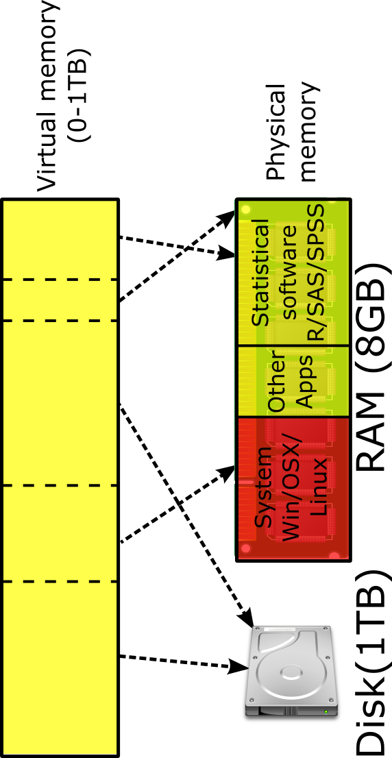
Memory mapping is based on the use of virtual memory. The virtual memory of a computer can be much greater than its RAM. Memory mapping associates a segment of virtual memory with the data file on the hard drive. In this way, it does not need to read the entire content of a data file into RAM but the part of data that are immediately needed. After the use of the part of the data, they are removed from RAM to allow another part of data to be used. This method is illustrated in the figure below. Note that the virtual memory can be as big as the disk space.
The R package bigmemory (Kane et al., 2013) uses the idea for data management. The package defines a new data structure/type called big.matrix for numeric matrices which uses memory-mapped files to allow matrices to exceed the RAM size. The underlying technology is memory mapping on modern operating systems that associates a segment of virtual memory in a one-to-one correspondence with the contents of a file. These files are accessed at a much faster speed than in the database approaches because operations are handled at the operating-system level.
The function read.big.matrix can be used to read the data. The function only supports one type of data - double, integer, short (large integer number), and char. It creates a pointer to the file created on the computer. Therefore, the object itself is extremely small.
b.names <- c('y', paste0('x', 1:44))
system.time(bigdata <- read.big.matrix('D:/data/bigdata1.txt', header=FALSE, type="double", sep=" ",
                           col.names=b.names, backingpath = "D:/data/", backingfile="bigdata.back",
                           descriptorfile="bigdata.desc"))
##    user  system elapsed
##  333.81   12.36  457.55


msize(bigdata)
## [1] "696 bytes"

describe(bigdata)
## An object of class "big.matrix.descriptor"
## Slot "description":
## $sharedType
## [1] "FileBacked"
##
## $filename
## [1] "bigdata.back"
##
## $dirname
## [1] "D:/data//"
##
## $totalRows
## [1] 9300000
##
## $totalCols
## [1] 45
##
## $rowOffset
## [1]       0 9300000
##
## $colOffset
## [1]  0 45
##
## $nrow
## [1] 9300000
##
## $ncol
## [1] 45
##
## $rowNames
## NULL
##
## $colNames
##  [1] "y"   "x1"  "x2"  "x3"  "x4"  "x5"  "x6"  "x7"  "x8"  "x9"  "x10" "x11"
## [13] "x12" "x13" "x14" "x15" "x16" "x17" "x18" "x19" "x20" "x21" "x22" "x23"
## [25] "x24" "x25" "x26" "x27" "x28" "x29" "x30" "x31" "x32" "x33" "x34" "x35"
## [37] "x36" "x37" "x38" "x39" "x40" "x41" "x42" "x43" "x44"
##
## $type
## [1] "double"
##
## $separated
## [1] FALSE
Many basic matrix operations can be used here.
dim(bigdata)
## [1] 9300000      45
head(bigdata)
##           y     x1     x2     x3     x4     x5     x6     x7    x8     x9
## [1,]  0.078  0.758 -0.694 -0.947 -2.581 -0.149 -0.200  1.964 0.326  0.992
## [2,]  2.698  2.123  0.131 -0.918  1.051 -0.701 -0.302  1.344 0.328 -0.490
## [3,] -0.504  0.357 -1.480 -0.426 -1.107  1.407 -0.847  1.979 0.230  0.673
## [4,] -0.886 -2.327 -0.480  1.080  1.882 -0.323 -0.913 -0.307 0.594  0.397
## [5,]  2.454  0.216  1.520  0.504 -0.471 -0.040 -0.333  0.446 0.105  0.041
## [6,]  1.520  0.877  0.769 -0.747 -0.044 -2.161 -0.106 -0.936 0.631  2.725
##         x10    x11    x12    x13    x14    x15    x16    x17   x18    x19
## [1,]  0.881  1.620  2.207  0.372  0.380  1.351  1.971  0.474 0.030  0.959
## [2,] -0.837 -0.658  0.950  0.123  1.191 -0.272  0.086  1.179 0.707 -0.891
## [3,] -0.601  0.242  1.543  0.206  0.241 -0.095  0.432 -0.243 0.265  2.195
## [4,] -0.522 -0.312 -3.415 -0.882  0.653  1.569 -1.102  0.391 0.364 -0.396
## [5,] -1.003 -0.684 -0.877  1.505 -1.629 -0.786  0.789 -0.139 0.798  1.873
## [6,] -0.075  1.933  0.722  0.680 -1.868 -2.974 -0.279 -1.296 1.544  0.992
##         x20    x21    x22    x23    x24    x25    x26    x27    x28    x29
## [1,] -0.675 -0.024 -0.102 -1.448 -1.158  0.010 -1.184 -0.572  0.520 -0.608
## [2,] -1.135  1.082 -0.332 -0.474 -0.974 -1.049  0.685 -0.203 -1.670 -0.783
## [3,]  2.175 -0.394  1.120 -0.834  2.391  2.097 -1.660  1.927 -0.349 -0.882
## [4,]  0.822  1.373 -1.385  1.044  1.144 -3.073  1.086 -0.516  0.310 -0.425
## [5,] -0.223 -1.333  0.846 -0.604 -2.525  0.082 -0.675 -0.807 -0.939 -0.258
## [6,]  0.385  0.222  0.130  0.757  0.011  0.187 -1.113 -1.004  0.104  0.542
##         x30    x31    x32    x33    x34    x35    x36    x37    x38    x39
## [1,] -0.547  0.598 -0.567  1.471 -1.067 -0.452  0.916  0.379 -0.943 -1.190
## [2,] -1.205 -1.230  0.500 -0.522 -0.007  1.652  0.104 -0.489 -0.823 -0.013
## [3,] -0.100  0.382 -1.084  0.136  0.331  0.413  0.103 -0.609  0.964  1.030
## [4,]  2.310  0.366 -0.739  0.434 -1.526 -0.196 -0.982 -1.372 -2.034 -0.480
## [5,] -0.024  0.141 -0.008  0.897  0.661 -0.503  1.255 -1.544  1.516 -0.702
## [6,]  0.393 -1.250 -0.277  0.155  0.188 -0.271  0.623  0.226  0.786  2.519
##         x40    x41    x42    x43    x44
## [1,] -0.086 -1.576 -0.600  1.452  0.189
## [2,]  0.324  0.257  1.557 -0.645  0.619
## [3,] -0.007  0.879 -0.585 -0.194  0.485
## [4,]  0.102 -2.111  0.036  1.363  0.696
## [5,]  0.281 -0.850  0.171 -0.182 -1.084
## [6,] -0.126 -0.134  2.008 -0.168 -0.428
tail(bigdata)
##           y     x1     x2     x3     x4     x5     x6     x7     x8     x9
## [1,]  0.729 -0.339  0.661 -2.108 -0.216 -1.969 -0.513 -1.534  1.916  0.128
## [2,]  3.097  0.852  0.994 -0.845 -0.890 -1.676  0.501 -0.982  0.352  0.180
## [3,] -2.146 -0.734 -1.307 -1.279  0.263 -0.522  1.943 -0.078  0.315  1.020
## [4,] -0.429 -0.912 -0.266 -0.498  0.268  0.308  2.106 -0.485 -0.725  0.087
## [5,]  0.076  0.249  0.638 -2.386  0.982  0.436 -1.811  0.944  0.863  1.285
## [6,] -0.589 -1.130 -1.445 -2.108 -0.604 -0.339 -0.428  0.211  1.997 -0.872
##         x10    x11    x12    x13    x14    x15    x16    x17    x18    x19
## [1,] -0.982  0.252  0.171  0.983 -0.562  2.201 -0.767  0.377  0.023 -1.258
## [2,] -1.083  1.152  0.662 -1.605 -0.038  1.721  0.244 -1.419 -1.391  1.383
## [3,] -0.036 -0.152 -1.717  1.417 -0.110 -0.681 -0.365 -1.846  0.115  0.998
## [4,]  1.295  1.012 -0.369 -0.538 -0.990  0.702 -1.941 -0.385  0.070 -0.366
## [5,]  0.404  1.326  0.882  1.211  0.090 -2.496  1.409 -1.835 -0.706 -1.323
## [6,] -0.206  1.149  1.074  0.756  0.425  0.368 -0.372  0.420 -0.182 -0.825
##         x20    x21    x22    x23    x24    x25    x26    x27    x28    x29
## [1,]  0.132  0.672 -1.082  0.548 -1.142 -1.172 -0.339 -0.359 -0.717  0.565
## [2,]  1.152  1.036  0.164 -1.465  1.693  0.049  0.100  0.652  0.154 -0.754
## [3,] -1.378 -0.021  0.454 -0.660  1.496  0.124 -0.746 -2.241  0.104 -0.916
## [4,]  1.422  1.110  1.276  0.106  0.207  0.670  0.174  0.430  0.195 -0.206
## [5,] -0.002  0.633  0.264 -1.761 -0.850  0.375  0.532  0.495  0.568  0.707
## [6,] -0.089  1.030 -0.477  0.164  0.512  0.743  0.549  0.029 -0.404 -0.908
##         x30    x31    x32    x33    x34    x35    x36    x37    x38    x39
## [1,]  1.115  2.267  0.990 -1.244 -1.005  0.679  0.437 -1.957 -1.598  0.586
## [2,]  0.208 -0.981 -1.784 -0.096 -0.461 -0.079 -1.562 -2.081  1.325 -1.201
## [3,]  0.536  1.913 -2.255 -0.083 -1.504  1.194 -1.493 -0.283 -1.039  0.147
## [4,] -1.599  0.977 -0.139  0.613 -0.264  0.498  1.153 -1.270 -2.702 -0.960
## [5,] -1.196  0.815  0.402 -1.129  1.084  0.315 -0.153 -0.317  0.123  1.279
## [6,] -0.289  0.109  0.364  0.190 -0.362  0.040 -0.753  0.482  0.660 -1.514
##         x40    x41    x42    x43    x44
## [1,]  0.058 -1.502 -1.122 -0.306  2.818
## [2,] -0.356 -0.505 -1.318  0.301 -0.873
## [3,]  0.111  0.064 -0.531  0.877  0.621
## [4,] -0.217  0.721 -1.785 -0.684 -0.007
## [5,] -0.578 -0.241 -1.507 -2.037 -0.404
## [6,] -0.748  0.213 -0.320  0.172 -0.956
summary(bigdata)
##               min           max          mean           NAs
## y   -6.986000e+00  6.772000e+00 -8.578753e-05  0.000000e+00
## x1  -5.203000e+00  4.978000e+00  1.032937e-04  0.000000e+00
## x2  -5.543000e+00  5.328000e+00  1.940722e-04  0.000000e+00
## x3  -5.152000e+00  5.002000e+00  4.110796e-04  0.000000e+00
## x4  -5.264000e+00  5.042000e+00 -3.704714e-04  0.000000e+00
## x5  -5.150000e+00  5.489000e+00  4.879371e-04  0.000000e+00
## x6  -5.218000e+00  5.176000e+00  3.849446e-04  0.000000e+00
## x7  -5.313000e+00  5.072000e+00  1.582546e-04  0.000000e+00
## x8  -4.980000e+00  5.306000e+00 -1.795616e-04  0.000000e+00
## x9  -5.335000e+00  5.447000e+00 -1.382226e-05  0.000000e+00
## x10 -5.328000e+00  5.118000e+00 -4.109939e-04  0.000000e+00
## x11 -4.945000e+00  4.991000e+00  1.364146e-04  0.000000e+00
## x12 -5.518000e+00  5.150000e+00 -2.684892e-04  0.000000e+00
## x13 -5.211000e+00  5.338000e+00 -3.417510e-04  0.000000e+00
## x14 -5.496000e+00  5.679000e+00 -1.890670e-04  0.000000e+00
## x15 -5.423000e+00  5.223000e+00 -1.623486e-04  0.000000e+00
## x16 -5.700000e+00  5.650000e+00  5.047738e-04  0.000000e+00
## x17 -5.133000e+00  5.235000e+00 -1.196059e-04  0.000000e+00
## x18 -5.071000e+00  4.996000e+00  4.349341e-04  0.000000e+00
## x19 -5.436000e+00  5.314000e+00 -1.393484e-05  0.000000e+00
## x20 -5.657000e+00  4.959000e+00 -2.316873e-04  0.000000e+00
## x21 -5.113000e+00  5.440000e+00 -3.070917e-04  0.000000e+00
## x22 -5.102000e+00  5.376000e+00  2.296577e-04  0.000000e+00
## x23 -4.998000e+00  5.271000e+00  1.018771e-04  0.000000e+00
## x24 -5.439000e+00  5.368000e+00  3.427799e-04  0.000000e+00
## x25 -4.996000e+00  5.060000e+00  8.001932e-04  0.000000e+00
## x26 -5.858000e+00  5.363000e+00  4.890148e-04  0.000000e+00
## x27 -5.434000e+00  5.569000e+00  1.631769e-04  0.000000e+00
## x28 -5.417000e+00  5.465000e+00 -8.578226e-05  0.000000e+00
## x29 -4.922000e+00  5.061000e+00 -1.692409e-05  0.000000e+00
## x30 -5.384000e+00  5.352000e+00 -9.349516e-05  0.000000e+00
## x31 -5.164000e+00  5.440000e+00 -1.631786e-04  0.000000e+00
## x32 -5.180000e+00  5.326000e+00  3.498729e-04  0.000000e+00
## x33 -5.239000e+00  5.015000e+00  2.694239e-04  0.000000e+00
## x34 -5.254000e+00  5.289000e+00  1.387848e-04  0.000000e+00
## x35 -5.249000e+00  5.246000e+00  2.275359e-04  0.000000e+00
## x36 -5.501000e+00  5.337000e+00 -8.486939e-04  0.000000e+00
## x37 -5.070000e+00  5.160000e+00  4.457989e-05  0.000000e+00
## x38 -5.597000e+00  4.912000e+00 -5.178778e-04  0.000000e+00
## x39 -5.336000e+00  5.226000e+00 -2.357135e-04  0.000000e+00
## x40 -5.405000e+00  5.145000e+00 -1.154631e-04  0.000000e+00
## x41 -5.107000e+00  5.251000e+00 -3.038226e-05  0.000000e+00
## x42 -5.432000e+00  5.296000e+00 -3.469746e-04  0.000000e+00
## x43 -4.999000e+00  5.262000e+00 -2.306269e-05  0.000000e+00
## x44 -4.954000e+00  5.032000e+00  4.638249e-04  0.000000e+00
The backing file is only created once. For example, once the data are read using read.big.matrix, we can further access the data in the following way. First, we can read the basic information from the .desc file. Then, we can attach the data in R using the attach.big.matrix function. Note that this takes almost no time.
# Read the pointer from disk .
bigdata.desc <- dget("D:/data/bigdata.desc")

# Attach to the pointer in RAM.
bigdata1 <- attach.big.matrix(bigdata.desc)
The R package biganalytics can be used to fit regression for big data.
library(biganalytics)
gc(reset = TRUE)
##              used    (Mb) gc trigger    (Mb)   max used    (Mb)
## Ncells   12606600   673.3   25020110  1336.3   12606600   673.3
## Vcells 2051326260 15650.4 4610729175 35177.1 2051326260 15650.4
big.lm.2 <- biglm.big.matrix(y ~ x1+x2+x3+x4+x5+x6+x7+x8+x9+x10+
                               x11+x12+x13+x14+x15+x16+x17+x18+x19+
                               x20+x21+x22+x23+x24+x25+x26+x27+x28+x29+
                               x30+x31+x32+x33+x34+x35+x36+x37+x38+x39+
                               x40+x41+x42+x43+x44, data = bigdata)
gc()
##              used    (Mb) gc trigger    (Mb)   max used    (Mb)
## Ncells   12609403   673.5   25020110  1336.3   25020110  1336.3
## Vcells 2051334182 15650.5 4610729175 35177.1 3957173940 30190.9
summary(big.lm.2)
## Large data regression model: biglm(formula = formula, data = data, ...)
## Sample size =  9300000
##                Coef    (95%     CI)    SE      p
## (Intercept) -0.0003 -0.0009  0.0004 3e-04 0.4169
## x1           0.8003  0.7996  0.8009 3e-04 0.0000
## x2           0.4999  0.4993  0.5006 3e-04 0.0000
## x3          -0.0005 -0.0011  0.0002 3e-04 0.1484
## x4          -0.0003 -0.0010  0.0004 3e-04 0.3570
## x5          -0.0005 -0.0011  0.0002 3e-04 0.1656
## x6          -0.0002 -0.0009  0.0005 3e-04 0.5524
## x7          -0.0002 -0.0009  0.0004 3e-04 0.4479
## x8           0.0003 -0.0003  0.0010 3e-04 0.3051
## x9           0.0005 -0.0002  0.0011 3e-04 0.1663
## x10         -0.0006 -0.0012  0.0001 3e-04 0.0783
## x11         -0.0001 -0.0008  0.0005 3e-04 0.6765
## x12         -0.0002 -0.0008  0.0005 3e-04 0.5746
## x13          0.0003 -0.0003  0.0010 3e-04 0.3349
## x14         -0.0003 -0.0009  0.0004 3e-04 0.4280
## x15         -0.0004 -0.0010  0.0003 3e-04 0.2681
## x16          0.0001 -0.0005  0.0008 3e-04 0.6734
## x17          0.0002 -0.0005  0.0009 3e-04 0.5366
## x18          0.0001 -0.0006  0.0007 3e-04 0.8653
## x19          0.0000 -0.0006  0.0007 3e-04 0.9181
## x20         -0.0009 -0.0016 -0.0003 3e-04 0.0041
## x21         -0.0001 -0.0008  0.0005 3e-04 0.7436
## x22          0.0005 -0.0002  0.0012 3e-04 0.1237
## x23         -0.0002 -0.0009  0.0004 3e-04 0.5021
## x24          0.0005 -0.0002  0.0011 3e-04 0.1361
## x25         -0.0001 -0.0008  0.0005 3e-04 0.7085
## x26          0.0000 -0.0007  0.0006 3e-04 0.8829
## x27         -0.0006 -0.0012  0.0001 3e-04 0.0930
## x28          0.0001 -0.0006  0.0007 3e-04 0.8194
## x29         -0.0007 -0.0013  0.0000 3e-04 0.0431
## x30         -0.0002 -0.0009  0.0005 3e-04 0.5462
## x31          0.0008  0.0001  0.0014 3e-04 0.0158
## x32         -0.0002 -0.0008  0.0005 3e-04 0.5935
## x33          0.0001 -0.0006  0.0008 3e-04 0.7676
## x34         -0.0001 -0.0008  0.0005 3e-04 0.6665
## x35          0.0005 -0.0001  0.0012 3e-04 0.1212
## x36         -0.0003 -0.0009  0.0004 3e-04 0.3821
## x37         -0.0002 -0.0009  0.0005 3e-04 0.5353
## x38         -0.0002 -0.0008  0.0005 3e-04 0.6204
## x39          0.0003 -0.0004  0.0010 3e-04 0.3606
## x40          0.0000 -0.0007  0.0007 3e-04 0.9917
## x41          0.0002 -0.0004  0.0009 3e-04 0.5045
## x42          0.0002 -0.0005  0.0008 3e-04 0.6014
## x43          0.0001 -0.0006  0.0007 3e-04 0.8068
## x44          0.0008  0.0001  0.0014 3e-04 0.0173
8.3.4 The ff and ffbase packages
The ff package works similarly like the bigmemory package but allows the mixture of different data types. The package ffbase extended ff with additive functions.
When using ff, it saves some information in a temporary directory.
# Get the temporary directory
getOption("fftempdir")
## [1] "C:/Users/zzhang4/AppData/Local/Temp/RtmpWe2ofB"

# Set new temporary directory
options(fftempdir = "D:/data")
We now again read the bigdata1.txt. Note that mulitple temporary files were created.
bigdata2 = read.table.ffdf(file="D:/data/bigdata1.txt", # File Name
                      sep=" ",         # Tab separator is used
                      header=FALSE,     # No variable names are included in the file
                      fill = TRUE,      # Missing values are represented by NA
                      )
Basic operation can be used like the bigmemory package.
names(bigdata2) <- c('y', paste0('x', 1:44))We save the ff data and then fast read it in the future.
ffsave(bigdata2,
       file="D:/data/bigdata1.ff",
       rootpath="D:/data")
##  [1] "  adding: ffdf2600195a3c0c.ff (172 bytes security) (deflated 69%)"
##  [2] "  adding: ffdf26005754a92.ff (172 bytes security) (deflated 70%)"
##  [3] "  adding: ffdf26002f6e2b5a.ff (172 bytes security) (deflated 70%)"
##  [4] "  adding: ffdf260050ba159d.ff (172 bytes security) (deflated 70%)"
##  [5] "  adding: ffdf260056e14795.ff (172 bytes security) (deflated 70%)"
##  [6] "  adding: ffdf260067384811.ff (172 bytes security) (deflated 70%)"
##  [7] "  adding: ffdf260019511d0.ff (172 bytes security) (deflated 70%)"
##  [8] "  adding: ffdf260066176ea5.ff (172 bytes security) (deflated 70%)"
##  [9] "  adding: ffdf260078b578a7.ff (172 bytes security) (deflated 70%)"
## [10] "  adding: ffdf260037b129ff.ff (172 bytes security) (deflated 70%)"
## [11] "  adding: ffdf26004fe54817.ff (172 bytes security) (deflated 70%)"
## [12] "  adding: ffdf2600183c1d2a.ff (172 bytes security) (deflated 70%)"
## [13] "  adding: ffdf26001c5db93.ff (172 bytes security) (deflated 70%)"
## [14] "  adding: ffdf26004daa2045.ff (172 bytes security) (deflated 70%)"
## [15] "  adding: ffdf2600153d4653.ff (172 bytes security) (deflated 70%)"
## [16] "  adding: ffdf260016cdb78.ff (172 bytes security) (deflated 70%)"
## [17] "  adding: ffdf2600339525f0.ff (172 bytes security) (deflated 70%)"
## [18] "  adding: ffdf260015bf2e2d.ff (172 bytes security) (deflated 70%)"
## [19] "  adding: ffdf2600fe0532e.ff (172 bytes security) (deflated 70%)"
## [20] "  adding: ffdf26003981467c.ff (172 bytes security) (deflated 70%)"
## [21] "  adding: ffdf260038ce4518.ff (172 bytes security) (deflated 70%)"
## [22] "  adding: ffdf26006ae2ce6.ff (172 bytes security) (deflated 70%)"
## [23] "  adding: ffdf260067474a53.ff (172 bytes security) (deflated 70%)"
## [24] "  adding: ffdf2600a22847.ff (172 bytes security) (deflated 70%)"
## [25] "  adding: ffdf260033ac3cac.ff (172 bytes security) (deflated 70%)"
## [26] "  adding: ffdf26003ed81e06.ff (172 bytes security) (deflated 70%)"
## [27] "  adding: ffdf2600306012f3.ff (172 bytes security) (deflated 70%)"
## [28] "  adding: ffdf26006591128f.ff (172 bytes security) (deflated 70%)"
## [29] "  adding: ffdf2600d87450c.ff (172 bytes security) (deflated 70%)"
## [30] "  adding: ffdf260012ba6e03.ff (172 bytes security) (deflated 70%)"
## [31] "  adding: ffdf26002a0d3643.ff (172 bytes security) (deflated 70%)"
## [32] "  adding: ffdf26007b40392d.ff (172 bytes security) (deflated 70%)"
## [33] "  adding: ffdf260035ea19e0.ff (172 bytes security) (deflated 70%)"
## [34] "  adding: ffdf26003f7546b9.ff (172 bytes security) (deflated 70%)"
## [35] "  adding: ffdf260049a55fb.ff (172 bytes security) (deflated 70%)"
## [36] "  adding: ffdf26005eb67ca0.ff (172 bytes security) (deflated 70%)"
## [37] "  adding: ffdf260017172892.ff (172 bytes security) (deflated 70%)"
## [38] "  adding: ffdf2600e4b51e7.ff (172 bytes security) (deflated 70%)"
## [39] "  adding: ffdf2600177252d9.ff (172 bytes security) (deflated 70%)"
## [40] "  adding: ffdf2600778e5489.ff (172 bytes security) (deflated 70%)"
## [41] "  adding: ffdf26005a824ed1.ff (172 bytes security) (deflated 70%)"
## [42] "  adding: ffdf2600214f4bb2.ff (172 bytes security) (deflated 70%)"
## [43] "  adding: ffdf26005b32331c.ff (172 bytes security) (deflated 70%)"
## [44] "  adding: ffdf26008784a2d.ff (172 bytes security) (deflated 70%)"
## [45] "  adding: ffdf26007d512910.ff (172 bytes security) (deflated 70%)"
To load the data into R, we use
ffload(file="D:/data/bigdata1.ff",
       overwrite = TRUE)
##  [1] "ffdf2600195a3c0c.ff" "ffdf26005754a92.ff"  "ffdf26002f6e2b5a.ff"
##  [4] "ffdf260050ba159d.ff" "ffdf260056e14795.ff" "ffdf260067384811.ff"
##  [7] "ffdf260019511d0.ff"  "ffdf260066176ea5.ff" "ffdf260078b578a7.ff"
## [10] "ffdf260037b129ff.ff" "ffdf26004fe54817.ff" "ffdf2600183c1d2a.ff"
## [13] "ffdf26001c5db93.ff"  "ffdf26004daa2045.ff" "ffdf2600153d4653.ff"
## [16] "ffdf260016cdb78.ff"  "ffdf2600339525f0.ff" "ffdf260015bf2e2d.ff"
## [19] "ffdf2600fe0532e.ff"  "ffdf26003981467c.ff" "ffdf260038ce4518.ff"
## [22] "ffdf26006ae2ce6.ff"  "ffdf260067474a53.ff" "ffdf2600a22847.ff"
## [25] "ffdf260033ac3cac.ff" "ffdf26003ed81e06.ff" "ffdf2600306012f3.ff"
## [28] "ffdf26006591128f.ff" "ffdf2600d87450c.ff"  "ffdf260012ba6e03.ff"
## [31] "ffdf26002a0d3643.ff" "ffdf26007b40392d.ff" "ffdf260035ea19e0.ff"
## [34] "ffdf26003f7546b9.ff" "ffdf260049a55fb.ff"  "ffdf26005eb67ca0.ff"
## [37] "ffdf260017172892.ff" "ffdf2600e4b51e7.ff"  "ffdf2600177252d9.ff"
## [40] "ffdf2600778e5489.ff" "ffdf26005a824ed1.ff" "ffdf2600214f4bb2.ff"
## [43] "ffdf26005b32331c.ff" "ffdf26008784a2d.ff"  "ffdf26007d512910.ff"
model_formula = as.formula(paste0("y ~", paste0(paste0('x',1:44), collapse="+")))
model_out = bigglm(model_formula, data=bigdata2)
summary(model_out)
## Large data regression model: bigglm(model_formula, data = bigdata2)
## Sample size = 9300000
## Coef (95% CI) SE p
## (Intercept) -0.0003 -0.0009 0.0004 3e-04 0.4169
## x1 0.8003 0.7996 0.8009 3e-04 0.0000
## x2 0.4999 0.4993 0.5006 3e-04 0.0000
## x3 -0.0005 -0.0011 0.0002 3e-04 0.1484
## x4 -0.0003 -0.0010 0.0004 3e-04 0.3570
## x5 -0.0005 -0.0011 0.0002 3e-04 0.1656
## x6 -0.0002 -0.0009 0.0005 3e-04 0.5524
## x7 -0.0002 -0.0009 0.0004 3e-04 0.4479
## x8 0.0003 -0.0003 0.0010 3e-04 0.3051
## x9 0.0005 -0.0002 0.0011 3e-04 0.1663
## x10 -0.0006 -0.0012 0.0001 3e-04 0.0783
## x11 -0.0001 -0.0008 0.0005 3e-04 0.6765
## x12 -0.0002 -0.0008 0.0005 3e-04 0.5746
## x13 0.0003 -0.0003 0.0010 3e-04 0.3349
## x14 -0.0003 -0.0009 0.0004 3e-04 0.4280
## x15 -0.0004 -0.0010 0.0003 3e-04 0.2681
## x16 0.0001 -0.0005 0.0008 3e-04 0.6734
## x17 0.0002 -0.0005 0.0009 3e-04 0.5366
## x18 0.0001 -0.0006 0.0007 3e-04 0.8653
## x19 0.0000 -0.0006 0.0007 3e-04 0.9181
## x20 -0.0009 -0.0016 -0.0003 3e-04 0.0041
## x21 -0.0001 -0.0008 0.0005 3e-04 0.7436
## x22 0.0005 -0.0002 0.0012 3e-04 0.1237
## x23 -0.0002 -0.0009 0.0004 3e-04 0.5021
## x24 0.0005 -0.0002 0.0011 3e-04 0.1361
## x25 -0.0001 -0.0008 0.0005 3e-04 0.7085
## x26 0.0000 -0.0007 0.0006 3e-04 0.8829
## x27 -0.0006 -0.0012 0.0001 3e-04 0.0930
## x28 0.0001 -0.0006 0.0007 3e-04 0.8194
## x29 -0.0007 -0.0013 0.0000 3e-04 0.0431
## x30 -0.0002 -0.0009 0.0005 3e-04 0.5462
## x31 0.0008 0.0001 0.0014 3e-04 0.0158
## x32 -0.0002 -0.0008 0.0005 3e-04 0.5935
## x33 0.0001 -0.0006 0.0008 3e-04 0.7676
## x34 -0.0001 -0.0008 0.0005 3e-04 0.6665
## x35 0.0005 -0.0001 0.0012 3e-04 0.1212
## x36 -0.0003 -0.0009 0.0004 3e-04 0.3821
## x37 -0.0002 -0.0009 0.0005 3e-04 0.5353
## x38 -0.0002 -0.0008 0.0005 3e-04 0.6204
## x39 0.0003 -0.0004 0.0010 3e-04 0.3606
## x40 0.0000 -0.0007 0.0007 3e-04 0.9917
## x41 0.0002 -0.0004 0.0009 3e-04 0.5045
## x42 0.0002 -0.0005 0.0008 3e-04 0.6014
## x43 0.0001 -0.0006 0.0007 3e-04 0.8068
## x44 0.0008 0.0001 0.0014 3e-04 0.01738.3.5 A divide and conque algorithm
For a very large data file on a computer, we can read a part of the data into R and conduct the analysis, and then combine the results together.
For the bigdata1.txt file, we can first inspect the first few rows of data and get the total number of rows of the data file.
readLines('D:/data/bigdata1.txt', n=3)
## [1] "0.078 0.758 -0.694 -0.947 -2.581 -0.149 -0.2 1.964 0.326 0.992 0.881 1.62 2.207 0.372 0.38 1.351 1.971 0.474 0.03 0.959 -0.675 -0.024 -0.102 -1.448 -1.158 0.01 -1.184 -0.572 0.52 -0.608 -0.547 0.598 -0.567 1.471 -1.067 -0.452 0.916 0.379 -0.943 -1.19 -0.086 -1.576 -0.6 1.452 0.189"
## [2] "2.698 2.123 0.131 -0.918 1.051 -0.701 -0.302 1.344 0.328 -0.49 -0.837 -0.658 0.95 0.123 1.191 -0.272 0.086 1.179 0.707 -0.891 -1.135 1.082 -0.332 -0.474 -0.974 -1.049 0.685 -0.203 -1.67 -0.783 -1.205 -1.23 0.5 -0.522 -0.007 1.652 0.104 -0.489 -0.823 -0.013 0.324 0.257 1.557 -0.645 0.619"
## [3] "-0.504 0.357 -1.48 -0.426 -1.107 1.407 -0.847 1.979 0.23 0.673 -0.601 0.242 1.543 0.206 0.241 -0.095 0.432 -0.243 0.265 2.195 2.175 -0.394 1.12 -0.834 2.391 2.097 -1.66 1.927 -0.349 -0.882 -0.1 0.382 -1.084 0.136 0.331 0.413 0.103 -0.609 0.964 1.03 -0.007 0.879 -0.585 -0.194 0.485"

#system('wc -l bigdata1.txt', intern = TRUE)

system('find /v /c "" D:/data/bigdata1.txt')
Now, suppose we would like to fit a regression model to the data. Instead of using all the data at one time, we only read in 10,000 rows of data each time. Therefore, we will do the analysis for 930 times.
## specify the first row of each reading of data
first.row <- seq(0, length=930, by=10000)
all.coef <- list()
for (i in 1:10){ ## change 10 to 930
  bg.subset <- read.table("D:/data/bigdata1.txt",
                        skip = first.row[i],
                        nrows= 10000,
                        header = FALSE)
  names(bg.subset) <- c('y', paste0('x', 1:44))
  model.subset <- lm(y~., data=bg.subset)
  all.coef[[i]] <- coef(model.subset)
  cat(i, "\n")
}
## 1
## 2
## 3
## 4
## 5
## 6
## 7
## 8
## 9
## 10

all.coef.matrix <- do.call(rbind, all.coef)
colMeans(all.coef.matrix)
##   (Intercept)            x1            x2            x3            x4
##  1.538501e-04  7.971463e-01  4.997889e-01  2.368758e-03 -2.127635e-03
##            x5            x6            x7            x8            x9
## -4.442199e-03  1.566934e-03  1.922532e-04  2.433141e-04  1.315510e-03
##           x10           x11           x12           x13           x14
##  2.349351e-04 -2.323344e-05 -1.482999e-03  3.138025e-03  3.163150e-04
##           x15           x16           x17           x18           x19
## -3.359310e-03  2.223121e-03  3.108206e-03 -2.669120e-03 -3.142849e-03
##           x20           x21           x22           x23           x24
## -2.291401e-03  3.418715e-03 -4.013795e-03 -3.270496e-03  2.510819e-03
##           x25           x26           x27           x28           x29
## -2.935929e-03 -9.711691e-06 -3.827271e-04  2.305276e-04  2.536062e-03
##           x30           x31           x32           x33           x34
##  2.261201e-03 -4.328551e-03  6.042383e-04  1.137028e-03  1.985576e-03
##           x35           x36           x37           x38           x39
##  2.730040e-03 -2.217446e-03 -2.185202e-03 -4.545015e-03  2.930815e-03
##           x40           x41           x42           x43           x44
##  1.609477e-03 -1.350481e-03  1.365137e-03 -1.974796e-03  7.837193e-04