Chapter 1 Introduction to R
1.1 What is R?
R is a programming language and free, open-source software environment for statistical computing and graphics. R is modeled after S and S-Plus (http://www.insightful.com). The S language was developed by John Chambers in 1976 in the late 1980s at AT&T labs. The R project was started by Robert Gentleman and Ross Ihaka of the Statistics Department of the University of Auckland in 1995. The first stable beta version R 1.0.0 was released in Feb 2000. R is named partly after the first names of the first two R authors and partly as a play on the name of S - ahead/better than S. The development of R is now supported by the R Foundation for Statistical Computing.
Although there are some important differences between S and R such as data and graphics formats, most common statistical functions programmed for S will run under R and vice-versa and much of the code written for S runs unaltered.
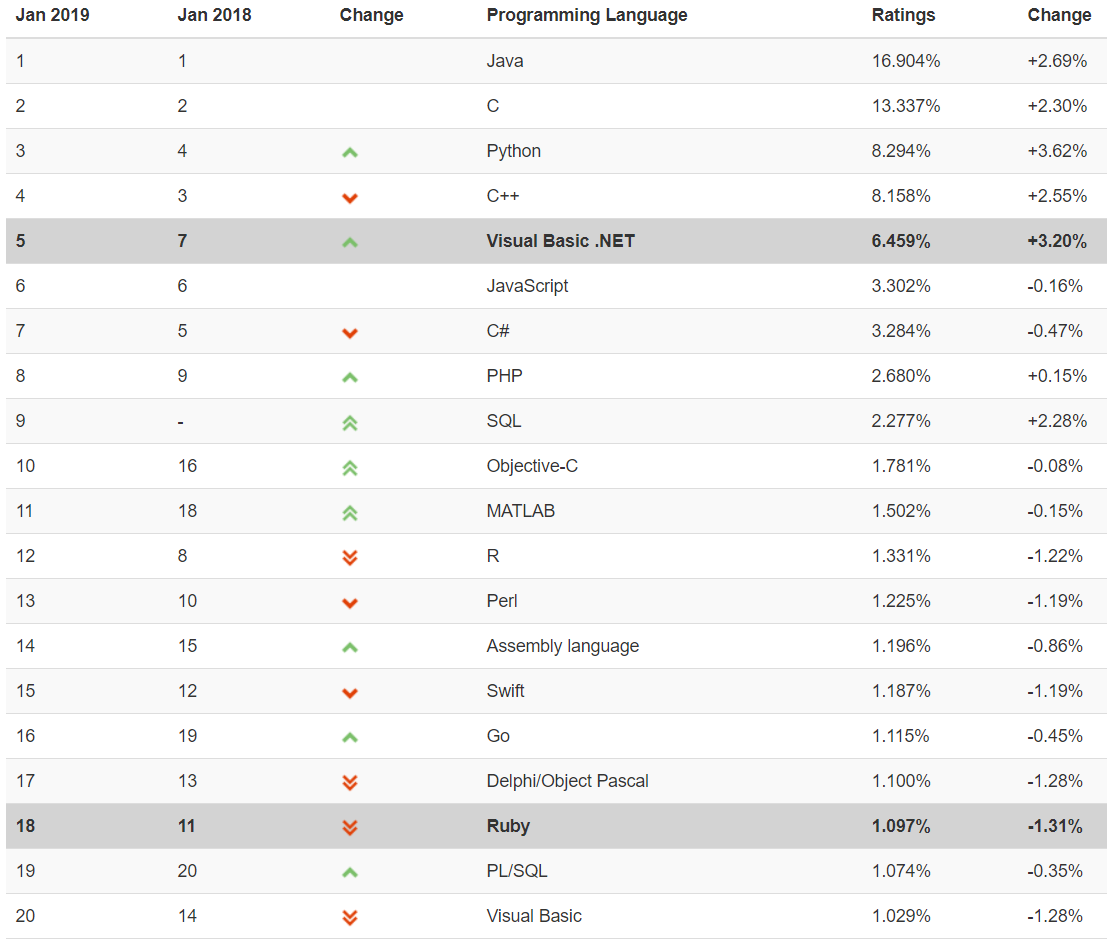
The R language is now widely used among statisticians and data miners for developing statistical software and data analysis. Based on the TIOBE index, a measure of the popularity of programming languages, R ranked the 12th in January 2019.
R is now maintained by a group of core researchers but with contributions from all over the world.
1.2 Install R
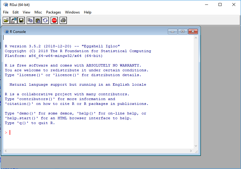
R consists of the base of R and contributed R packages. R and its packages are available on the Comprehensive R Archive Network (CRAN). There are many different mirrors of CRAN around the world. One can choose a mirror close to his/her location to download and install R. The URL of the original CRAN is https://cran.r-project.org. The base of R can be installed from its source code or compiled binaries for Windows, Mac OS X, and Linux.
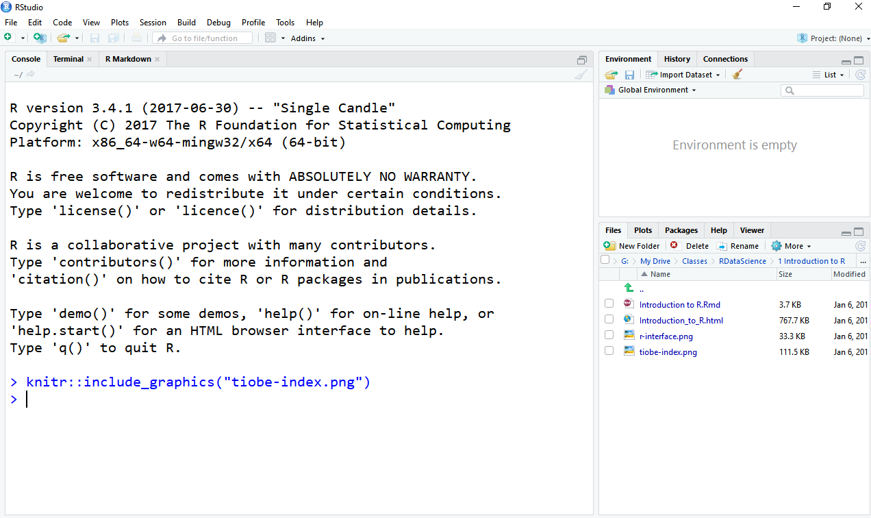
In addition to the basic implementation of R, there are also other environments built upon basic R. For example, RStudio is a free and open-source integrated development environment (IDE) for R. RStudio largely makes the use and development of R simpler. Particularly, it supports the seamless use of R through RMarkdown, knitr, and other packages. Microsoft R Open is an enhanced distribution of R from Microsoft Corporation. An earlier version of Microsoft R Open is Revolution R which is developed to focus on big data, large-scale multiprocessor computing, and multi-core functionality.
Because of the popularity of R, many other statistical packages have incorporated R for flexible data analysis. For example, SPSS can directly talk to R (see here). Similarly, one can also use R within SAS (see here).
In this class, we focus on the use of RStudio and the basic implementation of R. To download the software, use the links below:
1.3 Use R
After start R, it is most easily used in an interactive manner. You ask it a question and R gives you an answer. Questions are asked and answered on the command line. However, for more complex analysis or repetitive analysis, it is always more convenient to use a script file.
To start a new script file, one can simply use the menu of R. All the R related script and some other information can be typed in the script file. To run the R code, one can simply copy and paste it to the console or use the keyboard shortcuts such as control+enter in RStudio. One particular note is that anything after the character “#” is viewed as comments and ignored.
1.3.1 R markdown
R Markdown provides an authoring framework for data science. You can use a single R Markdown file to both
- save and execute code
- generate high quality reports that can be shared with an audience
For quick start, see https://www.rstudio.com/wp-content/uploads/2016/03/rmarkdown-cheatsheet-2.0.pdf
Some very basics:
- # starts a section
- Three ``` will insert any code.
- Three ```{r} will insert R code block.
- ` ` will insert inline R code
- - starts a list
1.3.2 Basic operations
R can be first used as an advanced calculator. The code below shows the use of addition (+), subtraction (-), multiplication (*), division (/), logarithm (ln), exponential (exp). 5
2+3
## [1] 5
4-1
## [1] 3
2*3
## [1] 6
(2+3)/4
## [1] 1.25
log(10)
## [1] 2.302585
exp(2)
## [1] 7.389056
5^3
## [1] 125
Each value used in R can be given a name and the value can be referred using its name. For example, if we let a = 2, then a can be used anywhere to replace the value 2. Some example code is given below.
a = 2
b <- 3
4 -> d

a*b
## [1] 6
(a+b)/d
## [1] 1.25
d^2
## [1] 16

(e=3)
## [1] 3
1.3.3 Vector
R is called a “vector language” because it can work on vectors directly. Vector is the most basic data structure in R. A vector is a collection of elements of the same data type. The data types can be logical, integer, double, character, complex or raw.
1.3.3.1 Create a vector
A vector can be created using the c() function, which combines its arguments or input to form a vector. Several examples are given below. As for the simple operations, names can be used for vectors. By typing its name, the content of a vector will be printed.
outcome <- c(1, 0, 0, 1, 0, 1)
gender <- c('F', 'F', 'M', 'F', 'M')
income <- c(100, 500, 900, 400, 700, 650, 320)

outcome
## [1] 1 0 0 1 0 1
gender
## [1] "F" "F" "M" "F" "M"
income
## [1] 100 500 900 400 700 650 320
Try out the typeof function.
typeof(outcome)
## [1] "double"
typeof(gender)
## [1] "character"
1.3.3.2 Operating a vector
1.3.3.2.1 Subset of a vector
Since there are multiple elements in a vector, the elements can be taken our using their index. The index of an element is its position in the vector. For example, the first element has the index 1, the second element has the index 2, and so on. For example, suppose there is a vector called income with 7 values: 100, 500, 900, 400, 700, 650, 320. To take out the first value, one can use income1 and to take out the last value, one can use income[7]. Note that the index is put into a set of brackets “[ ]”. A vector of indexes can be provided as a vector to take out multiple elements. For example, income[c(1, 3, 7)].
income <- c(100, 500, 900, 400, 700, 650, 320)
income[1]
## [1] 100
income[7]
## [1] 320
income[c(1,3,7)]
## [1] 100 900 320
income[2:5]
## [1] 500 900 400 700
1.3.3.2.2 Vector operations
A vector can be operated like a scalar in R. Most operations for a scalar will operate on all elements in a vector. For example, 2*income will multiply each element in income by 2. income > 500 will check each element to see whether it is larger than 500. The outcome is called a logical vector that includes values FALSE or TRUE. Some other examples can be seen below.
income <- c(100, 500, 900, 400, 700, 650, 320)
2*income
## [1]  200 1000 1800  800 1400 1300  640
income > 500
## [1] FALSE FALSE  TRUE FALSE  TRUE  TRUE FALSE
income == 500
## [1] FALSE  TRUE FALSE FALSE FALSE FALSE FALSE
income + 500
## [1]  600 1000 1400  900 1200 1150  820
income/10
## [1] 10 50 90 40 70 65 32
1.3.3.2.3 Basic statistical function operating on vectors
Since a vector is a collection of values, statistical functions can be applied to it. For example, the function length() tells the sample size (the number of elements) of a vector. The function sum() adds all the values in the vector together. Other functions include min(), max(), median(), sd(), var(), and many others.
income <- c(100, 500, 900, 400, 700, 650, 320)
length(income)
## [1] 7
summary(income)
##    Min. 1st Qu.  Median    Mean 3rd Qu.    Max.
##     100     360     500     510     675     900
min(income)
## [1] 100
max(income)
## [1] 900
median(income)
## [1] 500
sd(income)
## [1] 265.8947
var(income)
## [1] 70700
1.3.4 Array and Matrix
R saves a table of data in an array or a matrix. We usually deal with two-dimensional matrix but higher-dimensional matrix can also be used in R.
1.3.4.1 Create an array / matrix
Two functions can be used to create a matrix, array() or matrix(). We show how to create a 3 by 4 matrix.
The code below creates a matrix using the function array(). Note that 1:12 generates a sequence of values, 1, 2, …, 12. The sequence of values is used to create the matrix. dim=c(3,4) tells there are 3 rows and 4 columns in the matrix. The function takes the 12 values and fills each column sequentially. For example, it first fills in the first column using 1, 2, and 3. Then it fills the second column using 4, 5, and 6.
To change the positions of the values in the matrix, one has to change the input values. See the difference in the creation of matrix y.
x <- array(1:12, dim=c(3,4))
x
##      [,1] [,2] [,3] [,4]
## [1,]    1    4    7   10
## [2,]    2    5    8   11
## [3,]    3    6    9   12

y <- array(c(1,5,9,2,6,10,3,7,11,4,8,12), dim=c(3,4))
y
##      [,1] [,2] [,3] [,4]
## [1,]    1    2    3    4
## [2,]    5    6    7    8
## [3,]    9   10   11   12

z <- array(1:24, dim=c(2,3,4))
z
## , , 1
##
##      [,1] [,2] [,3]
## [1,]    1    3    5
## [2,]    2    4    6
##
## , , 2
##
##      [,1] [,2] [,3]
## [1,]    7    9   11
## [2,]    8   10   12
##
## , , 3
##
##      [,1] [,2] [,3]
## [1,]   13   15   17
## [2,]   14   16   18
##
## , , 4
##
##      [,1] [,2] [,3]
## [1,]   19   21   23
## [2,]   20   22   24
The function matrix() can control how to fill the values in a matrix. For example, setting byrow=TRUE, the values will be filled by rows instead of by columns. Note that to use the function, one needs to tell either the number of rows using nrow or the number of columns using ncol.
x <- matrix(1:12, nrow=3)
x
##      [,1] [,2] [,3] [,4]
## [1,]    1    4    7   10
## [2,]    2    5    8   11
## [3,]    3    6    9   12

y <- matrix(1:12, nrow=3, byrow=TRUE)
y
##      [,1] [,2] [,3] [,4]
## [1,]    1    2    3    4
## [2,]    5    6    7    8
## [3,]    9   10   11   12
1.3.4.2 Operating an array or matrix
We are often interested in taking out a subset of values in a matrix. x[i,j] takes out values according to the index i for the rows and j for the columns. Both i and j can be a single value or a vector. When i is replaced by blank, the whole column(s) is taken out and when j is replaced by blank, the whole row(s) is taken out. Some examples are given below.
Note that when a vector of values is taken out, by default, the sub-matrix will be converted to a vector and lose the matrix property. To keep the matrix property, add the option drop=FALSE.
x <- array(1:12, dim=c(3,4))
x
##      [,1] [,2] [,3] [,4]
## [1,]    1    4    7   10
## [2,]    2    5    8   11
## [3,]    3    6    9   12

x[2,3]
## [1] 8
x[1:2, 1:2]
##      [,1] [,2]
## [1,]    1    4
## [2,]    2    5
x[2, ]
## [1]  2  5  8 11
x[2, , drop=FALSE]
##      [,1] [,2] [,3] [,4]
## [1,]    2    5    8   11

x[, 3]
## [1] 7 8 9
x[, 3, drop=FALSE]
##      [,1]
## [1,]    7
## [2,]    8
## [3,]    9
1.3.5 List
A list is a collection of multiple objects which can be a scalar, a vector, a matrix, etc. Each object in a list can have its own name.
1.3.5.1 Create a list
To create a list, the function list() can be used as shown in the examples below.
x <- list('a'=3, 'b'=c(1,2), 'm'=array(1:6, dim=c(3,2)))
x
## $a
## [1] 3
##
## $b
## [1] 1 2
##
## $m
##      [,1] [,2]
## [1,]    1    4
## [2,]    2    5
## [3,]    3    6

a <- 3
b <- c(1,2)
m <- array(1:6, dim=c(3,2))

y <- list(a, b, m)
y
## [[1]]
## [1] 3
##
## [[2]]
## [1] 1 2
##
## [[3]]
##      [,1] [,2]
## [1,]    1    4
## [2,]    2    5
## [3,]    3    6
1.3.5.2 Access the object of a list
There are at least two ways to access the objects in a list. First, each object in the list has an index according to its order, which can be used to access that object. For example, x[1] will access the first object in the list. Note that [[ ]] instead of [ ] is used here. Second, the name of the object can be used to access it. For example, x$a will access a in the list. Note that a dollar sign $ is added between the name of the list and the name of the object.
x <- list('a'=3, 'b'=c(1,2), 'm'=array(1:6, dim=c(3,2)))

x[[3]]
##      [,1] [,2]
## [1,]    1    4
## [2,]    2    5
## [3,]    3    6

x$m
##      [,1] [,2]
## [1,]    1    4
## [2,]    2    5
## [3,]    3    6
1.3.6 Data frame
A data frame is a special list in which every object has the same size.
1.3.6.1 Create a data frame
To create a data frame, the function data.frame() can be used as shown in the examples below. The data read from a file into R are often saved into a data frame.
a <- 1:3
b <- 4:6
d <- 7:9
y <- data.frame(a,b,d)
y
##   a b d
## 1 1 4 7
## 2 2 5 8
## 3 3 6 9
1.3.6.2 Access the components of a data frame
The same methods for access the objects in a list can be used for a data frame. For example, y$a will access a in the data frame. The R function attach() can conveniently copy all objects in a data frame into R workspace so that they can be accessed using their names directly. To remove those objects, the function detach() can be used. Some examples are given below.
y <- data.frame(a=1:4,b=5:8,d=9:12)
y
##   a b  d
## 1 1 5  9
## 2 2 6 10
## 3 3 7 11
## 4 4 8 12

y$a
## [1] 1 2 3 4

attach(y)
b
## [1] 4 5 6

detach(y)
# b
# return an error
Note that to delete something from R console/memory, one can use the function rm().
y <- 3
y
## [1] 3

rm(y)
# y

# return an error
1.3.7 Generate data
Data can be generated or simulated in R. This can be useful when evaluating certain techniques with known data properties.
The function seq() can be used to generate a sequence of data
1:15
##  [1]  1  2  3  4  5  6  7  8  9 10 11 12 13 14 15
15:-3
##  [1] 15 14 13 12 11 10  9  8  7  6  5  4  3  2  1  0 -1 -2 -3

seq(from=0, to=5, by=.5)
##  [1] 0.0 0.5 1.0 1.5 2.0 2.5 3.0 3.5 4.0 4.5 5.0

seq(0, 1, length.out = 10)
##  [1] 0.0000000 0.1111111 0.2222222 0.3333333 0.4444444 0.5555556 0.6666667
##  [8] 0.7777778 0.8888889 1.0000000

seq(0, 1, length.out = 11)
##  [1] 0.0 0.1 0.2 0.3 0.4 0.5 0.6 0.7 0.8 0.9 1.0
We can randomly generate data from existing data using the function sample()
y <- 1:5

sample(y, size=3)
## [1] 2 1 3

sample(y, 5, replace = T)
## [1] 4 4 2 2 5

sample(y, 10, replace = T, prob=c(.05, .2, .3, .2, .05))
##  [1] 3 4 4 5 4 2 3 3 3 3
R also provides many functions to generate random numbers from a given distribution. These functions usually start with the letter “r”. For example, runif() for uniformly distributed random numbers and rnorm() for normally distributed random numbers.
runif(5, min=0, max=1)# from a uniform dist
## [1] 0.1258343 0.7208937 0.2974486 0.8872006 0.2110344

rnorm(5, mean=1, sd=2) # from a normal dist
## [1]  4.3045921  0.2676110 -0.2886091  1.5303316  0.6388332

rbinom(5,1,.3) # from a binomial dist
## [1] 1 0 0 0 0