Chapter 11 Log Analysis
In computer log management and intelligence, log analysis (or system and network log analysis) is an art and science seeking to make sense out of computer-generated records (also called log or audit trail records). The process of creating such records is called data logging.
For example, the website WebPower.psychstat.org hosts programs for statistical power analysis on an Apache Web server. When a user visits the website, the Apache server saves the log information into a log file called Apache access log file. One of such file is access-webpower.log.2.txt.
We first look at the log file with the first 5 lines shown below.
readLines("data/access-webpower.log.2.txt", n=5)
## [1] "54.36.148.177 - - [10/Feb/2019:06:51:02 -0500] \"GET /wiki/manual/relative_effect_size?idx=kb HTTP/1.1\" 200 7974 \"-\" \"Mozilla/5.0 (compatible; AhrefsBot/6.1; +http://ahrefs.com/robot/)\""
## [2] "192.3.9.217 - - [10/Feb/2019:06:52:17 -0500] \"GET /qanda/faq HTTP/1.0\" 200 7785 \"https://webpower.psychstat.org/\" \"Mozilla/5.0 (Windows; U; Windows NT 5.1; zh-CN) AppleWebKit/530.19.2 (KHTML, like Gecko) Version/4.0.2 Safari/530.19.1\""
## [3] "192.3.9.217 - - [10/Feb/2019:06:52:18 -0500] \"GET /qanda/register.php?redirect=qa%2Ffaq HTTP/1.1\" 404 6293 \"https://webpower.psychstat.org/\" \"Mozilla/5.0 (Windows; U; Windows NT 5.1; zh-CN) AppleWebKit/530.19.2 (KHTML, like Gecko) Version/4.0.2 Safari/530.19.1\""
## [4] "216.244.66.249 - - [10/Feb/2019:06:55:37 -0500] \"GET /robots.txt HTTP/1.1\" 200 3631 \"-\" \"Mozilla/5.0 (compatible; DotBot/1.1; http://www.opensiteexplorer.org/dotbot, help@moz.com)\""
## [5] "5.18.233.189 - - [10/Feb/2019:07:01:45 -0500] \"GET /wp-login.php HTTP/1.1\" 404 3957 \"-\" \"Mozilla/5.0 (Windows NT 6.1; WOW64; rv:40.0) Gecko/20100101 Firefox/40.1\""
The log file is in the following format: "%h %l %u %t \"%r\" %>s %b \"%{Referer}i\" \"%{User-agent}i\"" where
- %h is the remote host (ie the client IP)
- %l is the identity of the user determined by identd (not usually used since not reliable)
- %u is the user name determined by HTTP authentication
- %t is the time and time zone the request was received.
- %r is the request line from the client. (“GET / HTTP/1.0”)
- %>s is the status code sent from the server to the client (200, 404 etc.)
- %b is the size of the response to the client (in bytes)
- Referer is the Referer header of the HTTP request (containing the URL of the page from which this request was initiated) if any is present, and “-” otherwise.
- User-agent is the browser identification string.
Note that each component is separated by space. We now read the log file into R using the read.table function.
logfile <- read.table("data/access-webpower.log.2.txt", fill=TRUE, stringsAsFactors = FALSE)
dim(logfile)
## [1] 104544     10

## remove records with missing valus
logfile <- na.omit(logfile)
dim(logfile)
## [1] 104512     10

names(logfile) <- c("ip", "client", "user", "date.time", "time.zone",
                    "request", "status", "size", "referer", "user.agent")

head(logfile)
##               ip client user             date.time time.zone
## 1  54.36.148.177      -    - [10/Feb/2019:06:51:02    -0500]
## 2    192.3.9.217      -    - [10/Feb/2019:06:52:17    -0500]
## 3    192.3.9.217      -    - [10/Feb/2019:06:52:18    -0500]
## 4 216.244.66.249      -    - [10/Feb/2019:06:55:37    -0500]
## 5   5.18.233.189      -    - [10/Feb/2019:07:01:45    -0500]
## 6   5.18.233.189      -    - [10/Feb/2019:07:01:50    -0500]
##                                                 request status size
## 1 GET /wiki/manual/relative_effect_size?idx=kb HTTP/1.1    200 7974
## 2                               GET /qanda/faq HTTP/1.0    200 7785
## 3    GET /qanda/register.php?redirect=qa%2Ffaq HTTP/1.1    404 6293
## 4                              GET /robots.txt HTTP/1.1    200 3631
## 5                            GET /wp-login.php HTTP/1.1    404 3957
## 6                            GET /wp-login.php HTTP/1.1    404  502
##                           referer
## 1                               -
## 2 https://webpower.psychstat.org/
## 3 https://webpower.psychstat.org/
## 4                               -
## 5                               -
## 6                               -
##                                                                                                               user.agent
## 1                                                     Mozilla/5.0 (compatible; AhrefsBot/6.1; +http://ahrefs.com/robot/)
## 2 Mozilla/5.0 (Windows; U; Windows NT 5.1; zh-CN) AppleWebKit/530.19.2 (KHTML, like Gecko) Version/4.0.2 Safari/530.19.1
## 3 Mozilla/5.0 (Windows; U; Windows NT 5.1; zh-CN) AppleWebKit/530.19.2 (KHTML, like Gecko) Version/4.0.2 Safari/530.19.1
## 4                             Mozilla/5.0 (compatible; DotBot/1.1; http://www.opensiteexplorer.org/dotbot, help@moz.com)
## 5                                               Mozilla/5.0 (Windows NT 6.1; WOW64; rv:40.0) Gecko/20100101 Firefox/40.1
## 6                                               Mozilla/5.0 (Windows NT 6.1; WOW64; rv:40.0) Gecko/20100101 Firefox/40.1
A log file can be analyzed in different ways to identify useful information in it.
11.1 Where are the vistors from?
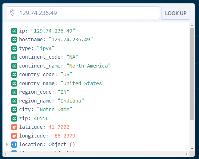
We can first see where the visitors to our website are from. This can be done based on the IP address in the log file. For example, the website https://ipstack.com/ provides an API to look up IP addresses. It provides geolocation information such as the latitude and longitude where the IP address is from.
From the log file, we first get all the IPs of the visitors.
iptable <- table(logfile$ip)
iptable <- data.frame(iptable)
names(iptable) <- c('ip', 'count')
iptable$ip <- as.character(iptable$ip)
head(iptable)
##             ip count
## 1 1.10.186.130     4
## 2 1.10.186.157     4
## 3 1.10.186.161     1
## 4 1.10.186.245     3
## 5 1.10.188.181     2
## 6 1.179.172.45     2
To use the API in R, one needs to register a (free) account to get an API key. For a free account, one can look up 10,000 IP address a month.
The following code is used to find the locations based on all the IPs in the log file. The IPs are saved in the file called ipinfo.RData.
## now get the geolocation information based on the ip address
## http://api.ipstack.com/129.74.236.49?access_key=70e2ed99b8adc82f911151f1d62e6e66

look.up.ip <- function(ip){
  url <- paste0("http://api.ipstack.com/", ip, "?access_key=70e2ed99b8adc82f911151f1d62e6e66")
  json.res <- fromJSON(url)
  json.res
}

ipinfo <- lapply(iptable$ip, look.up.ip)
save(ipinfo, file='ipinfo.RData')
We now load the geolocation information into R directly without resorting to the API.
load('data/ipinfo.RData')
ipinfo[1:2]
## [[1]]
## [[1]]$ip
## [1] "1.10.186.130"
##
## [[1]]$type
## [1] "ipv4"
##
## [[1]]$continent_code
## [1] "AS"
##
## [[1]]$continent_name
## [1] "Asia"
##
## [[1]]$country_code
## [1] "TH"
##
## [[1]]$country_name
## [1] "Thailand"
##
## [[1]]$latitude
## [1] "13.75"
##
## [[1]]$longitude
## [1] "100.4667"
##
## [[1]]$location.capital
## [1] "Bangkok"
##
## [[1]]$location.languages.code
## [1] "th"
##
## [[1]]$location.languages.name
## [1] "Thai"
##
## [[1]]$location.languages.native
## [1] "<U+0E44><U+0E17><U+0E22> / Phasa Thai"
##
## [[1]]$location.country_flag
## [1] "http://assets.ipstack.com/flags/th.svg"
##
## [[1]]$location.country_flag_emoji
## [1] "<U+0001F1F9><U+0001F1ED>"
##
## [[1]]$location.country_flag_emoji_unicode
## [1] "U+1F1F9 U+1F1ED"
##
## [[1]]$location.calling_code
## [1] "66"
##
## [[1]]$location.is_eu
## [1] "FALSE"
##
##
## [[2]]
## [[2]]$ip
## [1] "1.10.186.157"
##
## [[2]]$type
## [1] "ipv4"
##
## [[2]]$continent_code
## [1] "AS"
##
## [[2]]$continent_name
## [1] "Asia"
##
## [[2]]$country_code
## [1] "TH"
##
## [[2]]$country_name
## [1] "Thailand"
##
## [[2]]$latitude
## [1] "13.75"
##
## [[2]]$longitude
## [1] "100.4667"
##
## [[2]]$location.capital
## [1] "Bangkok"
##
## [[2]]$location.languages.code
## [1] "th"
##
## [[2]]$location.languages.name
## [1] "Thai"
##
## [[2]]$location.languages.native
## [1] "<U+0E44><U+0E17><U+0E22> / Phasa Thai"
##
## [[2]]$location.country_flag
## [1] "http://assets.ipstack.com/flags/th.svg"
##
## [[2]]$location.country_flag_emoji
## [1] "<U+0001F1F9><U+0001F1ED>"
##
## [[2]]$location.country_flag_emoji_unicode
## [1] "U+1F1F9 U+1F1ED"
##
## [[2]]$location.calling_code
## [1] "66"
##
## [[2]]$location.is_eu
## [1] "FALSE"
ipinfo.table <- rbindlist(ipinfo, fill=TRUE)
str(ipinfo.table)
## Classes 'data.table' and 'data.frame':   3395 obs. of  52 variables:
##  $ ip                                 : chr  "1.10.186.130" "1.10.186.157" "1.10.186.161" "1.10.186.245" ...
##  $ type                               : chr  "ipv4" "ipv4" "ipv4" "ipv4" ...
##  $ continent_code                     : chr  "AS" "AS" "AS" "AS" ...
##  $ continent_name                     : chr  "Asia" "Asia" "Asia" "Asia" ...
##  $ country_code                       : chr  "TH" "TH" "TH" "TH" ...
##  $ country_name                       : chr  "Thailand" "Thailand" "Thailand" "Thailand" ...
##  $ latitude                           : chr  "13.75" "13.75" "13.75" "13.75" ...
##  $ longitude                          : chr  "100.4667" "100.4667" "100.4667" "100.4667" ...
##  $ location.capital                   : chr  "Bangkok" "Bangkok" "Bangkok" "Bangkok" ...
##  $ location.languages.code            : chr  "th" "th" "th" "th" ...
##  $ location.languages.name            : chr  "Thai" "Thai" "Thai" "Thai" ...
##  $ location.languages.native          : chr  "<U+0E44><U+0E17><U+0E22> / Phasa Thai" "<U+0E44><U+0E17><U+0E22> / Phasa Thai" "<U+0E44><U+0E17><U+0E22> / Phasa Thai" "<U+0E44><U+0E17><U+0E22> / Phasa Thai" ...
##  $ location.country_flag              : chr  "http://assets.ipstack.com/flags/th.svg" "http://assets.ipstack.com/flags/th.svg" "http://assets.ipstack.com/flags/th.svg" "http://assets.ipstack.com/flags/th.svg" ...
##  $ location.country_flag_emoji        : chr  "<U+0001F1F9><U+0001F1ED>" "<U+0001F1F9><U+0001F1ED>" "<U+0001F1F9><U+0001F1ED>" "<U+0001F1F9><U+0001F1ED>" ...
##  $ location.country_flag_emoji_unicode: chr  "U+1F1F9 U+1F1ED" "U+1F1F9 U+1F1ED" "U+1F1F9 U+1F1ED" "U+1F1F9 U+1F1ED" ...
##  $ location.calling_code              : chr  "66" "66" "66" "66" ...
##  $ location.is_eu                     : chr  "FALSE" "FALSE" "FALSE" "FALSE" ...
##  $ region_code                        : chr  NA NA NA NA ...
##  $ region_name                        : chr  NA NA NA NA ...
##  $ city                               : chr  NA NA NA NA ...
##  $ zip                                : chr  NA NA NA NA ...
##  $ location.geoname_id                : chr  NA NA NA NA ...
##  $ location.languages.code1           : chr  NA NA NA NA ...
##  $ location.languages.code2           : chr  NA NA NA NA ...
##  $ location.languages.name1           : chr  NA NA NA NA ...
##  $ location.languages.name2           : chr  NA NA NA NA ...
##  $ location.languages.native1         : chr  NA NA NA NA ...
##  $ location.languages.native2         : chr  NA NA NA NA ...
##  $ location.languages.code3           : chr  NA NA NA NA ...
##  $ location.languages.code4           : chr  NA NA NA NA ...
##  $ location.languages.name3           : chr  NA NA NA NA ...
##  $ location.languages.name4           : chr  NA NA NA NA ...
##  $ location.languages.native3         : chr  NA NA NA NA ...
##  $ location.languages.native4         : chr  NA NA NA NA ...
##  $ location.languages.code5           : chr  NA NA NA NA ...
##  $ location.languages.code6           : chr  NA NA NA NA ...
##  $ location.languages.code7           : chr  NA NA NA NA ...
##  $ location.languages.code8           : chr  NA NA NA NA ...
##  $ location.languages.code9           : chr  NA NA NA NA ...
##  $ location.languages.code10          : chr  NA NA NA NA ...
##  $ location.languages.name5           : chr  NA NA NA NA ...
##  $ location.languages.name6           : chr  NA NA NA NA ...
##  $ location.languages.name7           : chr  NA NA NA NA ...
##  $ location.languages.name8           : chr  NA NA NA NA ...
##  $ location.languages.name9           : chr  NA NA NA NA ...
##  $ location.languages.name10          : chr  NA NA NA NA ...
##  $ location.languages.native5         : chr  NA NA NA NA ...
##  $ location.languages.native6         : chr  NA NA NA NA ...
##  $ location.languages.native7         : chr  NA NA NA NA ...
##  $ location.languages.native8         : chr  NA NA NA NA ...
##  $ location.languages.native9         : chr  NA NA NA NA ...
##  $ location.languages.native10        : chr  NA NA NA NA ...
##  - attr(*, ".internal.selfref")=<externalptr>
11.1.1 Visualization
We have identified the origin or countries of each visitor. Now, we plot the data. First, we generate a bar plot to show the number of visitors for the top 20 countries.
## display the raw number of visits
ipinfo.table %>%
  group_by(country_name) %>%
  summarise(counts = n()) %>%
  arrange(-counts) %>%
  top_n(20) %>%
  mutate(country_name = reorder(country_name, counts)) %>%
  ggplot(aes(x=country_name, y=counts)) +
    geom_bar(stat="identity") +
    coord_flip()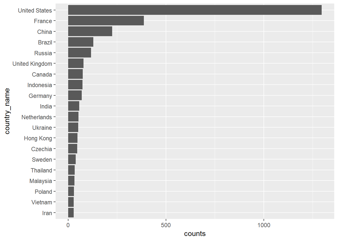
## display the percent of visitors for each country
ipinfo.table %>%
  group_by(country_name) %>%
  summarise(counts = n()) %>%
  arrange(-counts) %>%
  mutate(counts = counts/sum(counts)) %>%
  top_n(20) %>%
  mutate(country_name = reorder(country_name, counts)) %>%
  ggplot(aes(x=country_name, y=counts)) +
    geom_bar(stat="identity") +
    coord_flip()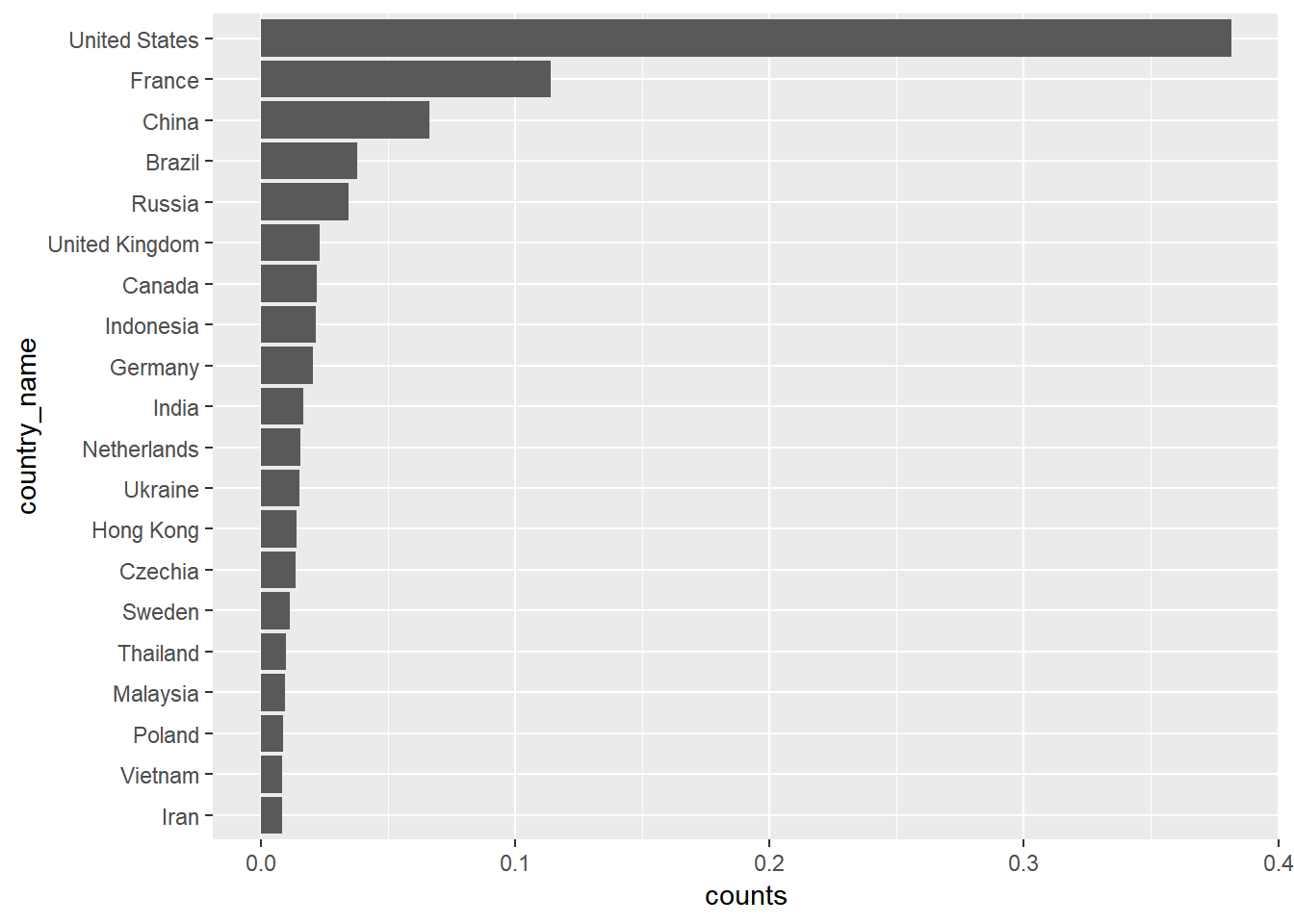
We now visualize the data on a map.
world <- map_data("world")
str(world)
## 'data.frame':    99338 obs. of  6 variables:
##  $ long     : num  -69.9 -69.9 -69.9 -70 -70.1 ...
##  $ lat      : num  12.5 12.4 12.4 12.5 12.5 ...
##  $ group    : num  1 1 1 1 1 1 1 1 1 1 ...
##  $ order    : int  1 2 3 4 5 6 7 8 9 10 ...
##  $ region   : chr  "Aruba" "Aruba" "Aruba" "Aruba" ...
##  $ subregion: chr  NA NA NA NA ...

w.map <- ggplot() + geom_polygon(data = world,
                        aes(x=long, y = lat, group = group, fill=region)) +
  coord_fixed(1.3) +
  guides(fill=FALSE)

w.map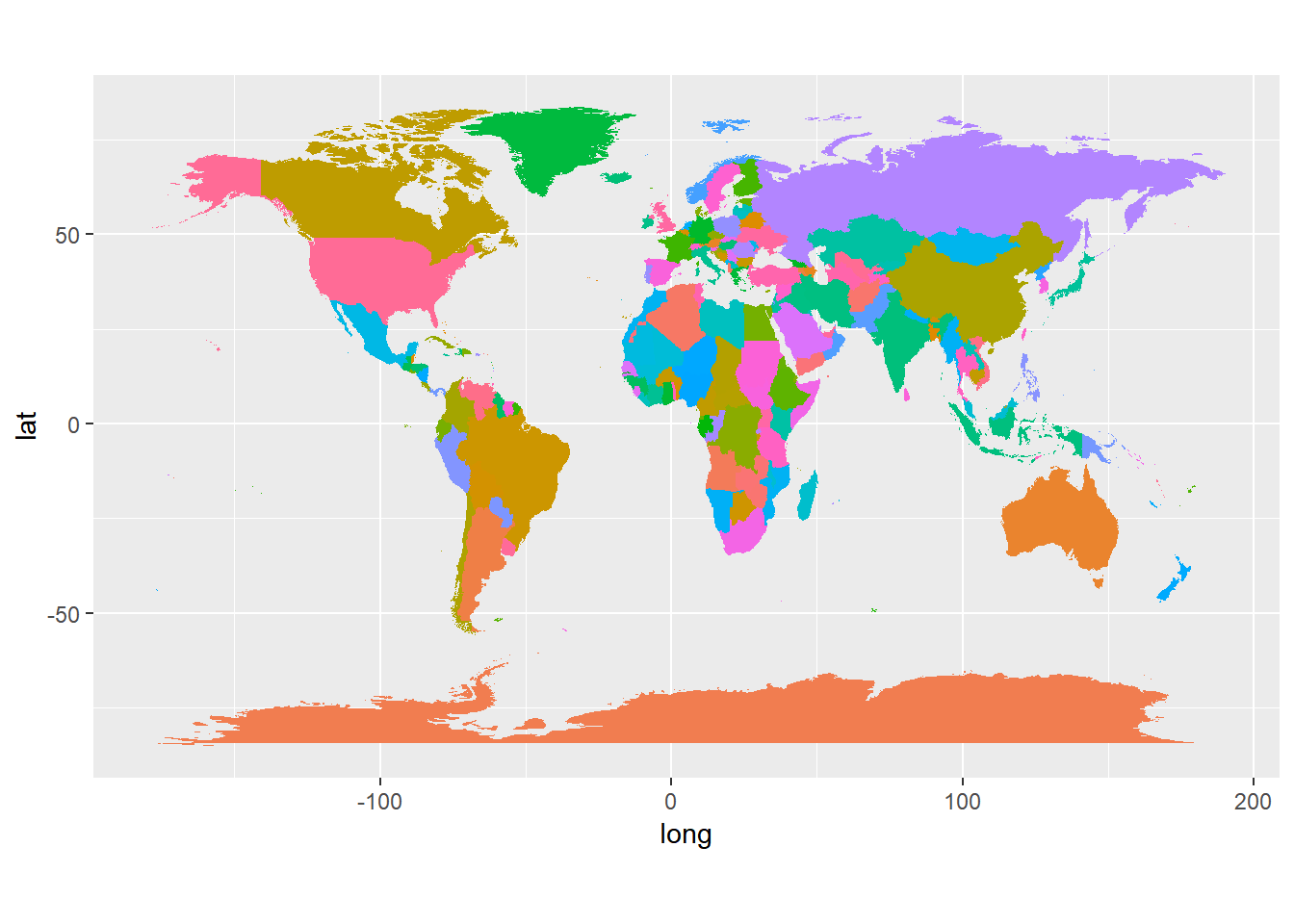
We now add the visitor information to it.
map.data <- ipinfo.table %>%
  group_by(country_name) %>%
  summarise(counts = n(), long = mean(as.numeric(longitude)), lat = mean(as.numeric(latitude))) %>%
  mutate(c.percent = counts/sum(counts)) %>%
  drop_na()

w.map +
   geom_point(data=map.data, aes(long, lat, size=counts))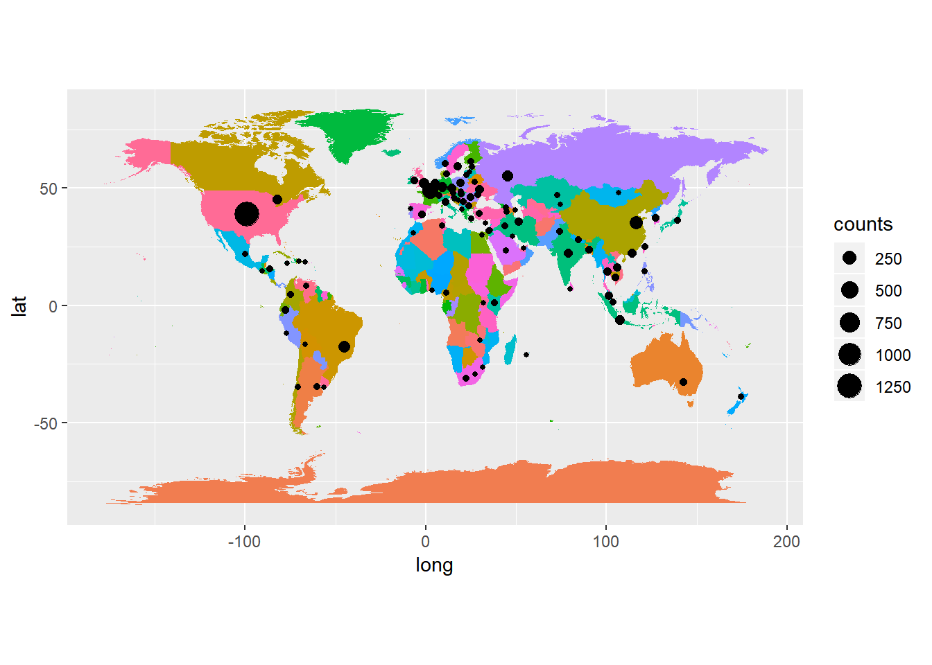
For the visitors from US, the state information is available. Therefore, we can display more detailed information.
usstates <- map_data('state')

usmap <- ggplot(data = usstates) +
  geom_polygon(aes(x = long, y = lat, fill = region, group = group), color = "white") +
  coord_fixed(1.3) +
  guides(fill=FALSE)

usmap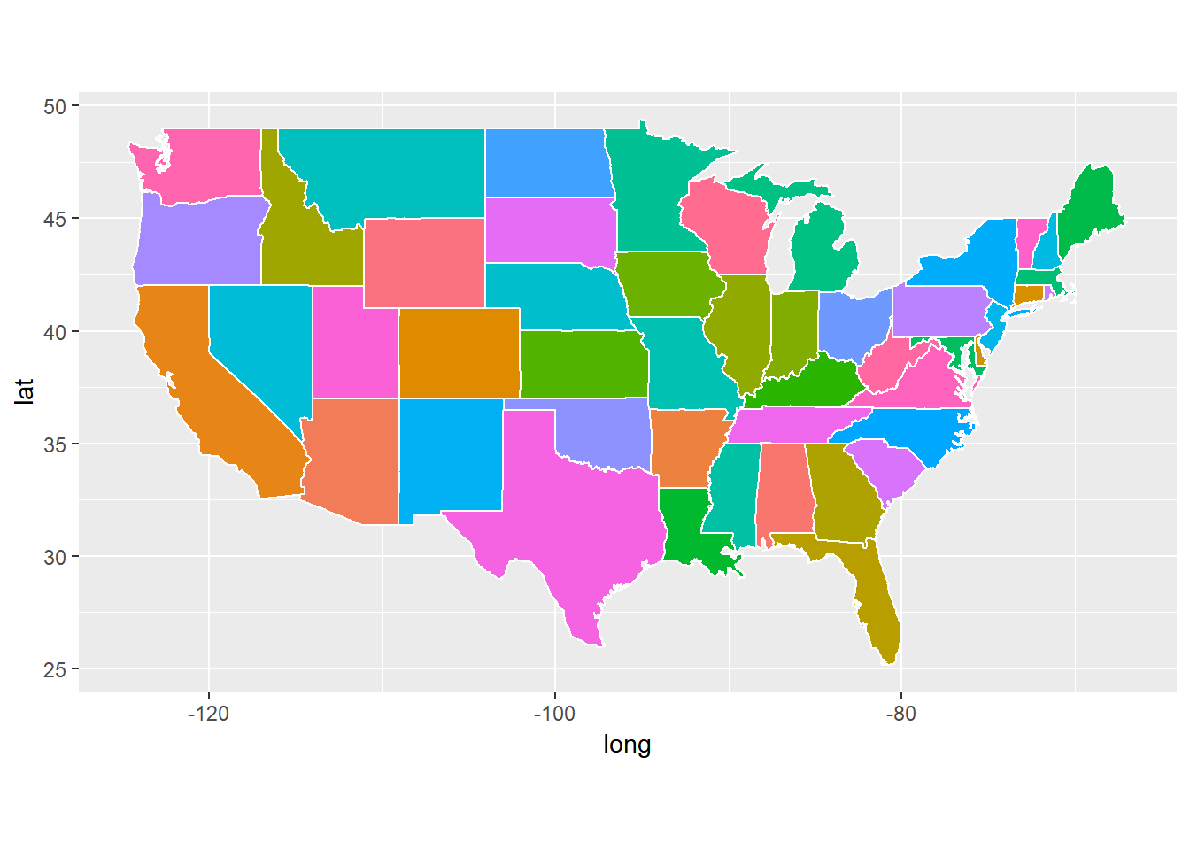
us.map.data <- ipinfo.table %>%
  filter(country_code == "US") %>%
  group_by(region_code) %>%
  summarise(counts = n(), long = mean(as.numeric(longitude)), lat = mean(as.numeric(latitude))) %>%
  mutate(c.percent = counts/sum(counts)) %>%
  drop_na() %>%
  filter(long > -140)

usmap + geom_point(data=us.map.data, aes(long, lat, size=counts))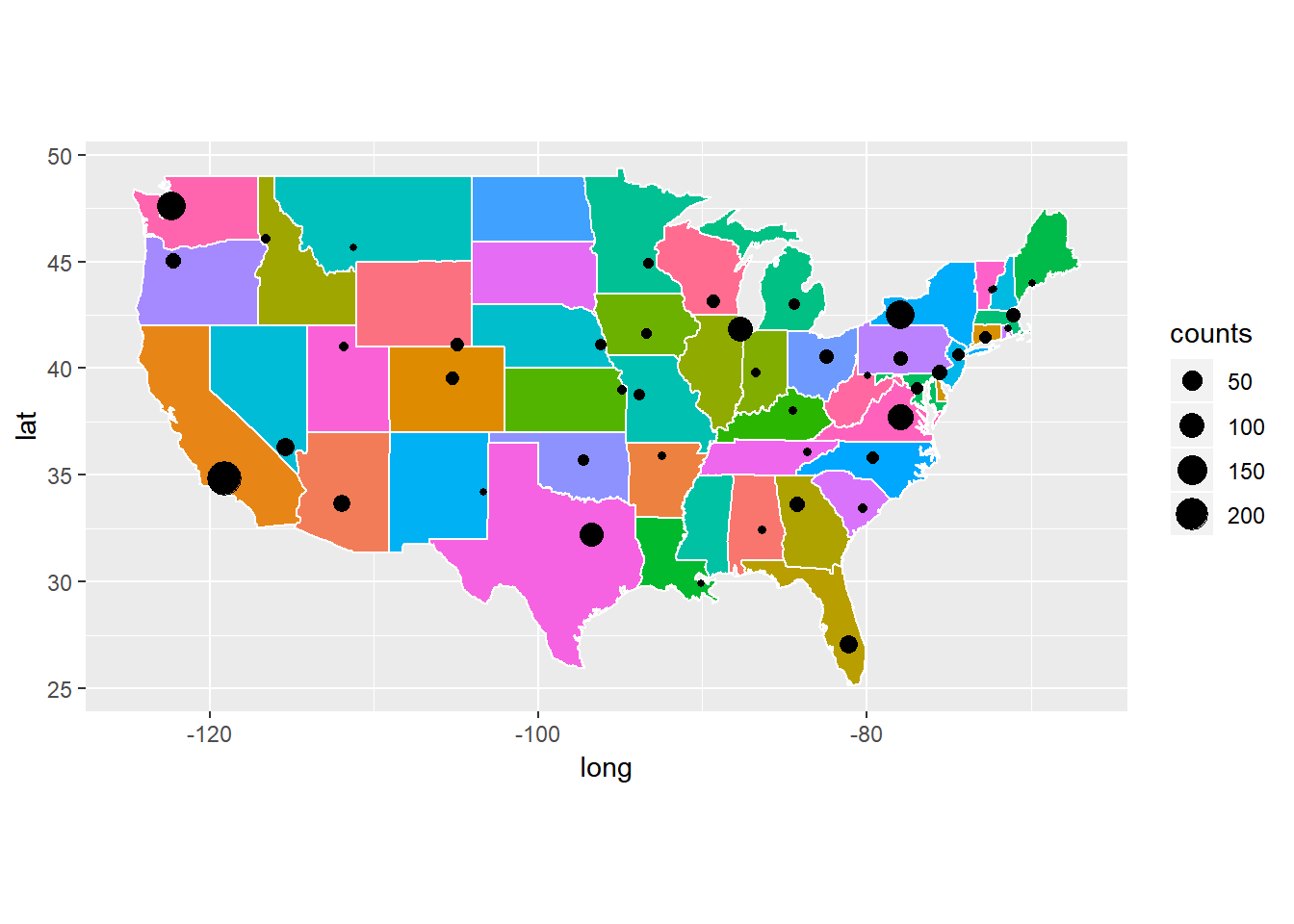
11.2 Vistors over time
We can see how the number of visitors change over time. To do so, we first convert the date and time to date format in R. For plotting later, we need to use the POSIXct format.
## change to date format
logfile$date.time <- as.POSIXct(strptime(logfile$date.time,"[%d/%b/%Y:%H:%M:%S"))

## time interval
logfile$date.time[104512] - logfile$date.time[1]
## Time difference of 7.52456 days

## truncate data to days and hours
logfile$dates <- as.POSIXct(trunc(logfile$date.time, units = "days"))
logfile$hours <- as.POSIXct(trunc(logfile$date.time, units = "hours"))
We now plot the number of page views over days.
page.view.day <- logfile %>%
  group_by(dates) %>%
  summarise(counts = n()) %>%
  drop_na()

ggplot(data=page.view.day, aes(x=dates, y=counts)) +
  geom_line() +
  geom_point()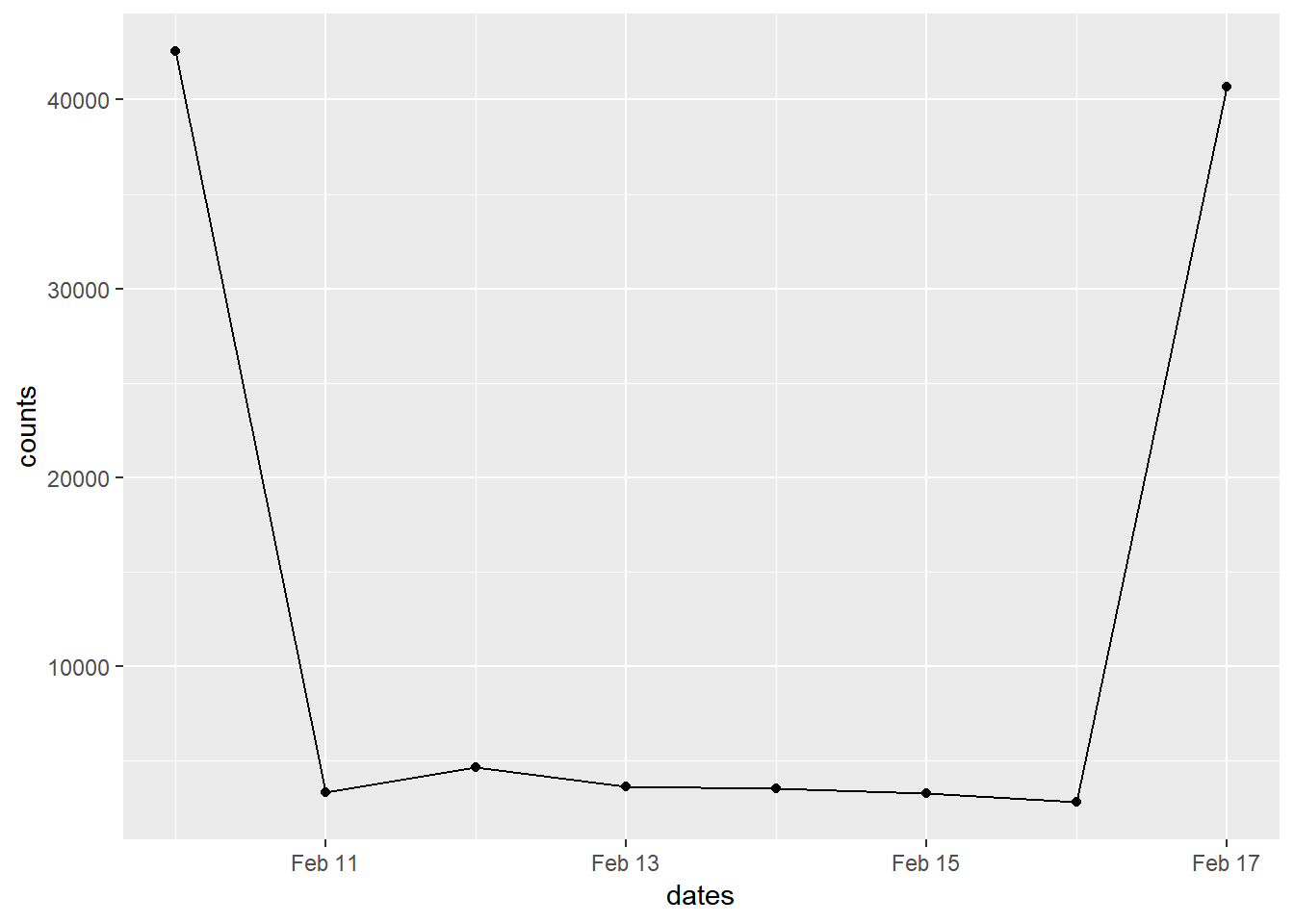
Another useful measure is how many unique visitors on each day. We then plot the unique IP each day.
page.view.day <- logfile %>%
  group_by(dates) %>%
  summarise(counts = length(unique(ip))) %>%
  drop_na()

ggplot(data=page.view.day, aes(x=as.Date(dates), y=counts)) +
  geom_line() +
  geom_point() +
  scale_x_date(date_breaks = 'day',
                 date_labels = '%b %d\n%a', name = 'Day')
11.2.1 More in-depth analysis
The log file includes the requested webpage. For the different models, the URL would have the components /models/.
## split the url
url <- strsplit(logfile$request, split="/")
## keep the ones with lengths < 10
url <-url[lengths(url) < 10]
## convert the list to a data frame
url <- plyr::ldply(url, rbind)
## choose the second column == 'models'
url <- url[url[, 2]=="models", 2:3]
names(url) <- c('models', 'type')
## plot the data
url %>%
  mutate(type = as.character(type)) %>%
  group_by(type) %>%
  summarise(counts = n()) %>%
  arrange(-counts) %>%
  mutate(type = reorder(type, counts)) %>%
  ggplot(aes(x=type, y=counts)) +
    geom_bar(stat="identity") +
    coord_flip()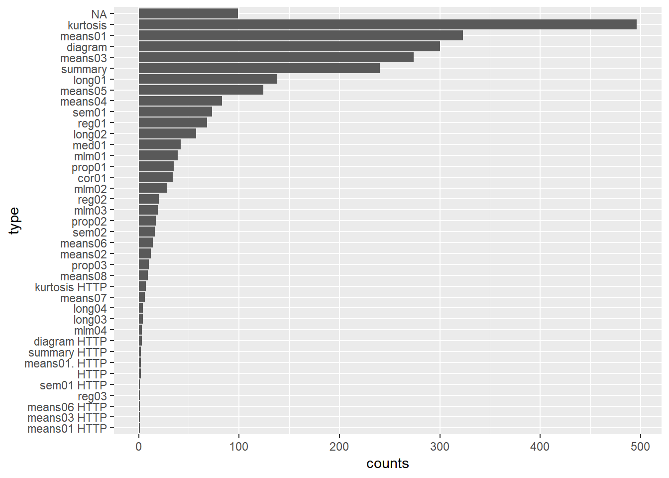
The referer
sum(str_detect(logfile$referer, "google"))
## [1] 765
sum(str_detect(logfile$referer, "wikipedia"))
## [1] 171
sum(str_detect(logfile$referer, "twitter"))
## [1] 3
sum(str_detect(logfile$referer, "facebook"))
## [1] 6
When requesting a webpage, it will first return with a status code such as 200, 404, and 500. Each code has a different meaning. For a complete list, see https://www.w3.org/Protocols/rfc2616/rfc2616-sec10.html.
- 10.2 Successful 2xx
- 200 OK The request has succeeded.
- 206 Partial Content
- Redirection 3xx
- Client Error 4xx
- 400 Bad Request
- 403 Forbidden
- 404 Not Found
- 405 Method Not Allowed
- Server Error 5xx
- 500 Internal Server Error
- 501 Not Implemented
table(as.numeric(logfile$status))
##
##   200   206   301   302   304   400   401   403   404   405   408   417   500
## 69387   338   641  4965    76   763     6   174 27007   594    60    32     9
##   501
##   428
11.2.2 More on client information
The log file also includes information on the types of operating systems and browsers used.
"Mozilla/5.0 (X11; Linux x86_64) AppleWebKit/537.36 (KHTML, like Gecko) Chrome/66.0.3359.139 Safari/537.36"
"Mozilla/5.0 (Windows NT 6.1; Win64; x64) AppleWebKit/537.36 (KHTML, like Gecko) Chrome/72.0.3626.96 Safari/537.36" "Mozilla/5.0 (Macintosh; U; Intel Mac OS X 10_6_8; en-us) AppleWebKit/534.50 (KHTML, like Gecko) Version/5.1 Safari/534.50"
"Mozilla/5.0 (compatible; DotBot/1.1; http://www.opensiteexplorer.org/dotbot, help@moz.com)"
First, we see how many accesses are from bots/spiders/crawlers.
bot <- str_detect(logfile$user.agent, "bot") | str_detect(logfile$user.agent, "spider") | str_detect(logfile$user.agent, "crawler")
sum(bot)
## [1] 4404

log.nonbot <- logfile[!bot, "user.agent"]
length(log.nonbot)
## [1] 100108
Then, we look at the type of operating systems, particularly mobile vs. desktop. Identifying this is actually more much difficult than it appears. For a list of user-agent used, see https://deviceatlas.com/blog/list-of-user-agent-strings.
Here, we simply search the user agent with the word “mob”.
mean(str_detect(logfile$user.agent, "[mM]ob"))
## [1] 0.01399839
Next, we look at different types of browsers.
mean(str_detect(logfile$user.agent, "Chrome"))
## [1] 0.1183692
mean(str_detect(logfile$user.agent, "Safari") & !str_detect(logfile$user.agent, "Chrome"))
## [1] 0.01932792
mean(str_detect(logfile$user.agent, "MSIE"))
## [1] 0.7540952
mean(str_detect(logfile$user.agent, "Firefox"))
## [1] 0.0332402
Finally, different types of OS.
mean(str_detect(logfile$user.agent, "Windows"))
## [1] 0.8321245
mean(str_detect(logfile$user.agent, "Linux"))
## [1] 0.05594573
mean(str_detect(logfile$user.agent, "Macintosh"))
## [1] 0.03540263
11.2.3 Maybe we should look at unique users instead.
distinct_log <- distinct(logfile, ip, .keep_all = TRUE)