Chapter 10 Market Basket Analysis
Market basket analysis is a type of affinity analysis that can be used to discover co-occurrence relationships among activities performed by (or recorded about) specific individuals or groups. In the market basket analysis, one seeks to understand the purchase behavior of customers. For example, if you are in a grocery store and you buy a 6-pack beer, you are more likely to buy a bag of chips at the same time than somebody who buys a dozen of eggs.
Each time a customer makes a purchase, it is referred to a transaction. The items bought in that transaction is referred to as an itemset. Market basket analysis investigates the combinations of items that occur together frequently in transactions to understand shopping behavior. This kind of analysis can be very helpful in retail. For example, in a grocery store, the items that are bought together frequently can be put close to each other. In online shopping, a website can recommend the associated items to customers.
10.1 Data
The data file groceries.csv contains 1 month (30 days) of real-world point-of-sale transaction data from a typical local grocery outlet. The data set contains 9,835 transactions and the items are aggregated to 169 categories, for example, by combining the same grocery of different brands.
The first 5 rows of data are shown below. Each row represents a transaction with different grocery items.
readLines('data/groceries.csv', n = 5)
## [1] "citrus fruit,semi-finished bread,margarine,ready soups"
## [2] "tropical fruit,yogurt,coffee"
## [3] "whole milk"
## [4] "pip fruit,yogurt,cream cheese ,meat spreads"
## [5] "other vegetables,whole milk,condensed milk,long life bakery product"
Although the data are in the .csv format, they are very different from typical data we see. Usually, we have the same number of columns and even when the number of columns is different, we would have the same information on the same column. Here, it is not the case. For example, if we use read.csv directly, we have
read.csv('data/groceries.csv', nrows=4, header=FALSE, fill = TRUE)
##               V1                  V2            V3           V4
## 1   citrus fruit semi-finished bread     margarine  ready soups
## 2 tropical fruit              yogurt        coffee
## 3     whole milk
## 4      pip fruit              yogurt cream cheese  meat spreads
Note that although we successfully read the data into 4 variables, it will cause problems in data analysis. This is because we would hope to have a matrix in the following format: Each row would represent a transaction and each column represents a type of grocery. Therefore, we would expect a 9835 by 169 matrix. Since rarely people would buy all 169 items a time, most likely a few items only, such a matrix is expected to be sparse.
The R package arules can be used to conduct market basket analysis. It also includes a function to read such data into a sparse matrix.
grocery <- read.transactions('data/groceries.csv', sep=',')
grocery
## transactions in sparse format with
##  9835 transactions (rows) and
##  169 items (columns)
str(grocery)
## Formal class 'transactions' [package "arules"] with 3 slots
##   ..@ data       :Formal class 'ngCMatrix' [package "Matrix"] with 5 slots
##   .. .. ..@ i       : int [1:43367] 29 88 118 132 33 157 167 166 38 91 ...
##   .. .. ..@ p       : int [1:9836] 0 4 7 8 12 16 21 22 27 28 ...
##   .. .. ..@ Dim     : int [1:2] 169 9835
##   .. .. ..@ Dimnames:List of 2
##   .. .. .. ..$ : NULL
##   .. .. .. ..$ : NULL
##   .. .. ..@ factors : list()
##   ..@ itemInfo   :'data.frame':  169 obs. of  1 variable:
##   .. ..$ labels: chr [1:169] "abrasive cleaner" "artif. sweetener" "baby cosmetics" "baby food" ...
##   ..@ itemsetInfo:'data.frame':  0 obs. of  0 variables
summary(grocery)
## transactions as itemMatrix in sparse format with
##  9835 rows (elements/itemsets/transactions) and
##  169 columns (items) and a density of 0.02609146
##
## most frequent items:
##       whole milk other vegetables       rolls/buns             soda
##             2513             1903             1809             1715
##           yogurt          (Other)
##             1372            34055
##
## element (itemset/transaction) length distribution:
## sizes
##    1    2    3    4    5    6    7    8    9   10   11   12   13   14   15   16
## 2159 1643 1299 1005  855  645  545  438  350  246  182  117   78   77   55   46
##   17   18   19   20   21   22   23   24   26   27   28   29   32
##   29   14   14    9   11    4    6    1    1    1    1    3    1
##
##    Min. 1st Qu.  Median    Mean 3rd Qu.    Max.
##   1.000   2.000   3.000   4.409   6.000  32.000
##
## includes extended item information - examples:
##             labels
## 1 abrasive cleaner
## 2 artif. sweetener
## 3   baby cosmetics
From the output, we see there are a total of 9,836 transactions and a total of 169 different groceries. The density of the matrix is about 2.6%. The most frequently bought item is whole milk, then other vegetables. We can also see that the majority of transactions has 10 items or less. In fact, there are 2,159 transactions with only one item. But there is also 1 transaction with 32 items.
inspect(grocery[size(grocery)==32])
##     items
## [1] {beef,
##      beverages,
##      butter,
##      candles,
##      chicken,
##      citrus fruit,
##      cream cheese,
##      curd,
##      domestic eggs,
##      flour,
##      frankfurter,
##      ham,
##      hard cheese,
##      hygiene articles,
##      liver loaf,
##      margarine,
##      mayonnaise,
##      other vegetables,
##      pasta,
##      roll products,
##      rolls/buns,
##      root vegetables,
##      sausage,
##      skin care,
##      soft cheese,
##      soups,
##      specialty fat,
##      sugar,
##      tropical fruit,
##      whipped/sour cream,
##      whole milk,
##      yogurt}
10.2 Association rules
The purpose of market basket analysis is often to identify association rules among items and this can be done through the Apriori algorithm. An association rule implies that if an item A occurs, then item B also occurs with a certain probability. Using the grocery data as an example.
| Transaction | Items |
|---|---|
| t1 | {citrus fruit,semi-finished bread,margarine,ready soups} |
| t2 | {tropical fruit,yogurt,coffee} |
| t3 | {pip fruit,yogurt,cream cheese ,meat spreads} |
In the table above we can see three transactions. Each transaction shows items bought in that transaction. We can represent our items as an item set as follows:
\[I=\{i_1, i_2,..., i_k\}\] where \(k\) is the total number of items such as grocery items.
For the grocery data, we have
\[I=\text{\{citrus fruit, semi-finished bread, margarine, ready soups, tropical fruit, yogurt, coffee ...\}}\]
A transaction is represented by the following expression:
\[T=\{t_1, t_2,..., t_n\}\] where \(n\) is the number items in this transaction. For example,
\[t_1=\text{\{citrus fruit, semi-finished bread, margarine, ready soups\}}\]
Then, an association rule is defined as an implication of the form:
For example,
\[\text{\{tropical fruit, yogurt\}} \Rightarrow \{coffee\}.\]
However, whether such a rule is plausible or not needs evaluation. To do so, we can use the following measures - support, confidence, lift, and conviction.
10.2.1 Support
Support is an indication of how frequently the itemset appears in the data set.
\[supp(X \& Y)=\dfrac{|X \cup Y|}{n} = P(X \& Y)\]
In other words, it’s the number of transactions with both \(X\) and \(Y\) divided by the total number of transactions. For example, for the grocery data.
\(supp(citrus\ fruit)=\frac{814}{9835} = 8.3\%\)
\(supp(citrus\ fruit \& margarine)=\frac{78}{9835}= 0.8 \%\)
\(supp(beef\ \& \ other\ vegetables \& root\ vegetables)=\frac{78}{9835} = 0.8 \%\)
grocery.text <- readLines('data/groceries.csv')

sum(str_detect(grocery.text, "citrus fruit"))
## [1] 814

sum(str_detect(grocery.text, "citrus fruit") & str_detect(grocery.text, "margarine"))
## [1] 78
sum(str_detect(grocery.text, "beef") & str_detect(grocery.text, "other vegetables") & str_detect(grocery.text, "root vegetables"))
## [1] 78
10.2.2 Confidence
Confidence is an indication of how often the rule has been found to be true. For a rule \(X \Rightarrow Y\), it means given \(X\), what is the probability to have \(Y\) in the same comment/transaction. This is called confidence. Confidence is like a conditional probability and it is an indication of how often the rule has been found to be true.
\[conf(X \Rightarrow Y)=\dfrac{supp(X \cup Y)}{supp(X)} = \frac{P(X \& Y)}{P(X)}.\]
For example, if a shopper bought “citrus fruit”, the confidence for the shopper to also buy “margarine” is
- \(conf(\text{citrus fruit } \Rightarrow \text{ margarine})=\dfrac{\frac{78}{9835}}{\frac{814}{9835}}= 9.6\%\)
mean(str_detect(grocery.text, "citrus fruit") & str_detect(grocery.text, "margarine")) / mean(str_detect(grocery.text, "citrus fruit"))
## [1] 0.0958231
10.2.3 Lift
The lift of a rule is the ratio of the observed confidence of \(X \Rightarrow Y\) to the support of \(Y\), and is defined as
\[lift(X \Rightarrow Y)=\dfrac{supp(X \cup Y)}{supp(X)supp(Y) }.\]
In other words, the lift is the ratio between observing \(Y\) given \(X\) to observing \(Y\) only. Another way to interpret it is that the ratio between \(X\) and \(Y\) together and \(X\) and \(Y\) independently. If the ratio is greater than 1, then it means it is more likely \(X\) and \(Y\) will be bought together than each individually. Therefore, greater lift values indicate stronger associations.
If the rule had a lift of 1, it would imply that the probability of occurrence of the antecedent and that of the consequent are independent of each other. When two events are independent of each other, no rule can be drawn involving those two events.
If the lift is > 1, that lets us know the degree to which those two occurrences are dependent on one another, and makes those rules potentially useful for predicting the consequent in future data sets.
If the lift is < 1, that lets us know the items are a substitute to each other. This means that the presence of one item has a negative effect on the presence of the other item and vice versa.
- \(lift(\text{citrus fruit } \Rightarrow \text{ margarine})=1.64\)
mean(str_detect(grocery.text, "citrus fruit") & str_detect(grocery.text, "margarine")) / (mean(str_detect(grocery.text, "citrus fruit")) * mean(str_detect(grocery.text, "margarine")))
## [1] 1.636146
10.2.4 Conviction
The conviction of a rule is defined as
\[conv(X \Rightarrow Y)=\dfrac{1-supp(Y)}{1-conf(X \Rightarrow Y) }\]
It can be interpreted as the ratio of the expected frequency that \(X\) occurs without \(Y\) (that is to say, the frequency that the rule makes an incorrect prediction) if \(X\) and \(Y\) were independent divided by the observed frequency of incorrect predictions. A high value means that the consequent depends strongly on the antecedent.
- \(conv(\text{citrus fruit } \Rightarrow \text{ margarine})= =1.01\)
In this example, the conviction value of 1.01 shows that the rule \(\text{citrus fruit } \Rightarrow \text{ margarine}\) would be incorrect 1% more often (1.01 times as often) if the association between citrus fruit and margarine was purely random chance.
(1 - mean(str_detect(grocery.text, "citrus fruit") )) /(1 - mean(str_detect(grocery.text, "citrus fruit") & str_detect(grocery.text, "margarine")) / mean(str_detect(grocery.text, "citrus fruit")))
## [1] 1.014441
10.3 Basic visualization
First, we can plot the frequent items using the function itemFrequencyPlot(). The code below plots the top 20 most frequently bought items.
itemFrequencyPlot(grocery, topN=20,
                  type="absolute",
                  horiz=TRUE)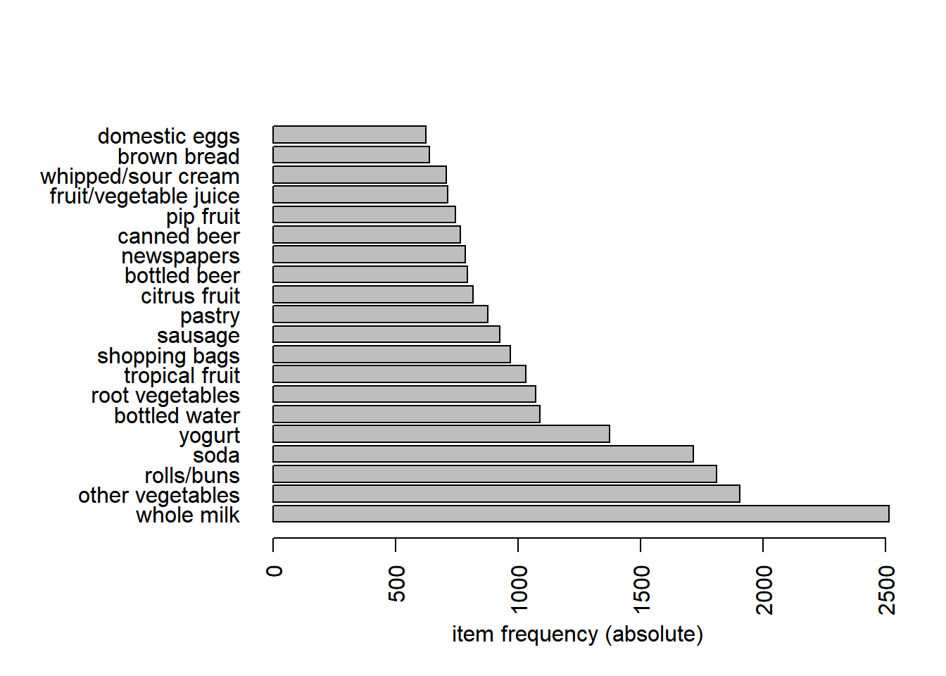
The itemFrequencyPlot() allows us to show the absolute or relative values. If absolute it will plot numeric frequencies of each item independently. If ‘relative’ it will plot how many times these items have appeared as compared to others, as it’s shown in the following plot.
itemFrequencyPlot(grocery, topN=20,
                  type="relative",
                  horiz=TRUE)
“Whole milk” is the best-selling product, followed by other vegetables and rolls/buns.
We can also visualize the transaction data using the level plot. Each row represents one transaction with a dot representing an item in that transaction.
image(grocery[1:200], aspect='fill')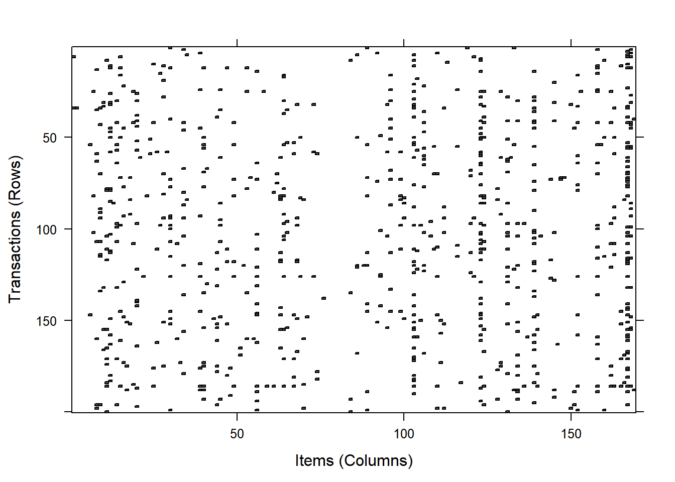 We can also randomly select a sample to visualize.
image(sample(grocery, 100), aspect='fill')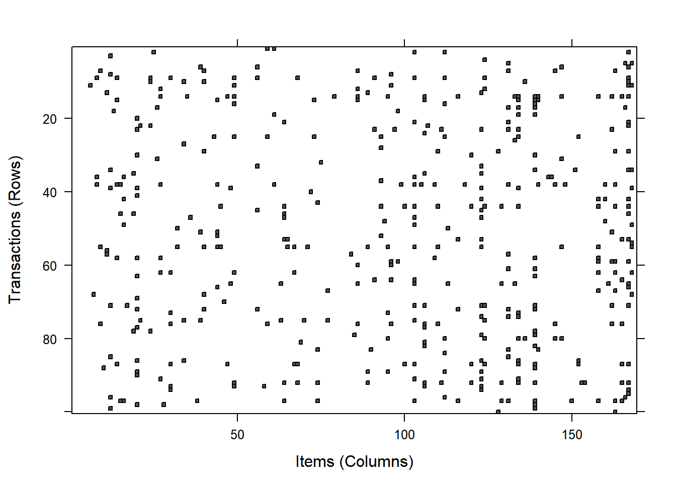
itemLabels(grocery)[168:169]
## [1] "yogurt"   "zwieback"
10.4 Apriori algorithm
The function apriori can be used to identify the association rules. To use the function, we need to make a choice on the support and confidence parameters. If we set these values too low, then the algorithm will take longer to execute, and we will get a lot of rules and most of them will not be useful. On the other hand, if we set these values too high, then the algorithm will get very few rules and miss some meaningful rules. The default behavior is to mine rules with minimum support of 0.1 and minimum confidence of 0.8.
The R generates rules in the following format:
LHS => RHS {A} => {B}
Apriori only creates rules with one item in the RHS (Consequent). The default value in the function parameter for minlen is 1. This means that rules with only one item (i.e., an empty antecedent/LHS) like
{} => {beer}
will be created. These rules mean that no matter what other items are involved, the item in the RHS will appear with the probability given by the rule’s confidence (which equals the support). If you want to avoid these rules then use the argument parameter=list(minlen=2).
If the minimum support is chosen too low for the dataset, then the algorithm will try to create an extremely large set of itemsets/rules. This will result in very long run time and eventually the process will run out of memory. To prevent this, the default maximal length of itemsets/rules is restricted to 10 items (via the parameter element maxlen=10) and the time for checking subsets is limited to 5 seconds (via maxtime=5). The output will show if you hit these limits in the “checking subsets” line of the output. The time limit is only checked when the subset size increases, so it may run significantly longer than what you specify in maxtime. Setting maxtime=0 disables the time limit.
Here we simply set support=0.005 and confidence = 0.25.
rules.set1 <- apriori(grocery,
                      parameter = list(supp=0.01,
                                       conf=0.25,
                                       minlen=2))
## Apriori
##
## Parameter specification:
##  confidence minval smax arem  aval originalSupport maxtime support minlen
##        0.25    0.1    1 none FALSE            TRUE       5    0.01      2
##  maxlen target   ext
##      10  rules FALSE
##
## Algorithmic control:
##  filter tree heap memopt load sort verbose
##     0.1 TRUE TRUE  FALSE TRUE    2    TRUE
##
## Absolute minimum support count: 98
##
## set item appearances ...[0 item(s)] done [0.00s].
## set transactions ...[169 item(s), 9835 transaction(s)] done [0.01s].
## sorting and recoding items ... [88 item(s)] done [0.00s].
## creating transaction tree ... done [0.01s].
## checking subsets of size 1 2 3 4 done [0.00s].
## writing ... [170 rule(s)] done [0.00s].
## creating S4 object  ... done [0.00s].
rules.set1
## set of 170 rules
The above specification leads to 170 rules. Basic information about the rules is given below.
summary(rules.set1)
## set of 170 rules
##
## rule length distribution (lhs + rhs):sizes
##  2  3
## 96 74
##
##    Min. 1st Qu.  Median    Mean 3rd Qu.    Max.
##   2.000   2.000   2.000   2.435   3.000   3.000
##
## summary of quality measures:
##     support          confidence          lift            count
##  Min.   :0.01007   Min.   :0.2517   Min.   :0.9932   Min.   : 99.0
##  1st Qu.:0.01159   1st Qu.:0.2973   1st Qu.:1.5215   1st Qu.:114.0
##  Median :0.01454   Median :0.3587   Median :1.7784   Median :143.0
##  Mean   :0.01822   Mean   :0.3703   Mean   :1.8747   Mean   :179.2
##  3rd Qu.:0.02097   3rd Qu.:0.4253   3rd Qu.:2.1453   3rd Qu.:206.2
##  Max.   :0.07483   Max.   :0.5862   Max.   :3.2950   Max.   :736.0
##
## mining info:
##     data ntransactions support confidence
##  grocery          9835    0.01       0.25
We can show the first few rules. The first rule means that if one buys “hard cheese”, he/she will also buy “whole milk”. The support of it is 0.01, meaning in 1% of the transactions, the two times were bought together. The confidence is 41% meaning that in transactions with “hard cheese”, 41% also bought “whole milk”. The lift is 1.61. This means comparing to overall shoppers who bought “whole milk”, the shoppers who bought “hard cheese” will lift the possibility to buy whole milk 61%.
inspect(rules.set1[1:10])
##      lhs                rhs                support    confidence lift     count
## [1]  {hard cheese}   => {whole milk}       0.01006609 0.4107884  1.607682  99
## [2]  {butter milk}   => {other vegetables} 0.01037112 0.3709091  1.916916 102
## [3]  {butter milk}   => {whole milk}       0.01159126 0.4145455  1.622385 114
## [4]  {ham}           => {whole milk}       0.01148958 0.4414062  1.727509 113
## [5]  {sliced cheese} => {whole milk}       0.01077783 0.4398340  1.721356 106
## [6]  {oil}           => {whole milk}       0.01128622 0.4021739  1.573968 111
## [7]  {onions}        => {other vegetables} 0.01423488 0.4590164  2.372268 140
## [8]  {onions}        => {whole milk}       0.01209964 0.3901639  1.526965 119
## [9]  {berries}       => {yogurt}           0.01057448 0.3180428  2.279848 104
## [10] {berries}       => {other vegetables} 0.01026945 0.3088685  1.596280 101
We can order the rules, too.
inspect(sort(rules.set1)[1:10])
##      lhs                   rhs                support    confidence lift
## [1]  {other vegetables} => {whole milk}       0.07483477 0.3867578  1.513634
## [2]  {whole milk}       => {other vegetables} 0.07483477 0.2928770  1.513634
## [3]  {rolls/buns}       => {whole milk}       0.05663447 0.3079049  1.205032
## [4]  {yogurt}           => {whole milk}       0.05602440 0.4016035  1.571735
## [5]  {root vegetables}  => {whole milk}       0.04890696 0.4486940  1.756031
## [6]  {root vegetables}  => {other vegetables} 0.04738180 0.4347015  2.246605
## [7]  {yogurt}           => {other vegetables} 0.04341637 0.3112245  1.608457
## [8]  {tropical fruit}   => {whole milk}       0.04229792 0.4031008  1.577595
## [9]  {tropical fruit}   => {other vegetables} 0.03589222 0.3420543  1.767790
## [10] {bottled water}    => {whole milk}       0.03436706 0.3109476  1.216940
##      count
## [1]  736
## [2]  736
## [3]  557
## [4]  551
## [5]  481
## [6]  466
## [7]  427
## [8]  416
## [9]  353
## [10] 338

inspect(sort(rules.set1, by='lift')[1:10])
##      lhs                                  rhs                support
## [1]  {citrus fruit,other vegetables}   => {root vegetables}  0.01037112
## [2]  {other vegetables,tropical fruit} => {root vegetables}  0.01230300
## [3]  {beef}                            => {root vegetables}  0.01738688
## [4]  {citrus fruit,root vegetables}    => {other vegetables} 0.01037112
## [5]  {root vegetables,tropical fruit}  => {other vegetables} 0.01230300
## [6]  {other vegetables,whole milk}     => {root vegetables}  0.02318251
## [7]  {curd,whole milk}                 => {yogurt}           0.01006609
## [8]  {other vegetables,yogurt}         => {root vegetables}  0.01291307
## [9]  {other vegetables,yogurt}         => {tropical fruit}   0.01230300
## [10] {other vegetables,rolls/buns}     => {root vegetables}  0.01220132
##      confidence lift     count
## [1]  0.3591549  3.295045 102
## [2]  0.3427762  3.144780 121
## [3]  0.3313953  3.040367 171
## [4]  0.5862069  3.029608 102
## [5]  0.5845411  3.020999 121
## [6]  0.3097826  2.842082 228
## [7]  0.3852140  2.761356  99
## [8]  0.2974239  2.728698 127
## [9]  0.2833724  2.700550 121
## [10] 0.2863962  2.627525 120
We can also identify rules that are related to a specific item.
citrus.rules <- subset(rules.set1, items %in% "citrus fruit")
inspect(citrus.rules)
##     lhs                                rhs                support    confidence
## [1] {citrus fruit}                  => {yogurt}           0.02165735 0.2616708
## [2] {citrus fruit}                  => {other vegetables} 0.02887646 0.3488943
## [3] {citrus fruit}                  => {whole milk}       0.03050330 0.3685504
## [4] {citrus fruit,root vegetables}  => {other vegetables} 0.01037112 0.5862069
## [5] {citrus fruit,other vegetables} => {root vegetables}  0.01037112 0.3591549
## [6] {citrus fruit,yogurt}           => {whole milk}       0.01026945 0.4741784
## [7] {citrus fruit,whole milk}       => {yogurt}           0.01026945 0.3366667
## [8] {citrus fruit,other vegetables} => {whole milk}       0.01301474 0.4507042
## [9] {citrus fruit,whole milk}       => {other vegetables} 0.01301474 0.4266667
##     lift     count
## [1] 1.875752 213
## [2] 1.803140 284
## [3] 1.442377 300
## [4] 3.029608 102
## [5] 3.295045 102
## [6] 1.855768 101
## [7] 2.413350 101
## [8] 1.763898 128
## [9] 2.205080 128
We can use the arulesViz package to visualize association rules. Let’s begin with a simple scatter plot with different measures of interestingness on the axes (lift and support) and a third measure (confidence) represented by the color of the points.
plot(rules.set1, measure=c("support","lift"), shading="confidence")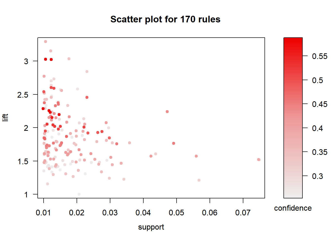
The following visualization represents the rules as a graph with items as labeled vertices, and rules represented as vertices connected to items using arrows.
# Graph
plot(rules.set1, method="graph")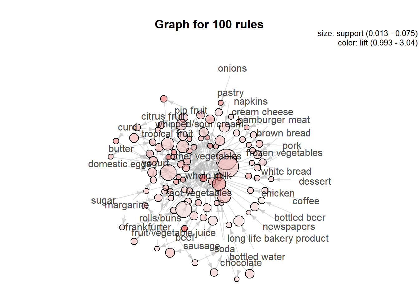
plot(citrus.rules, method="graph")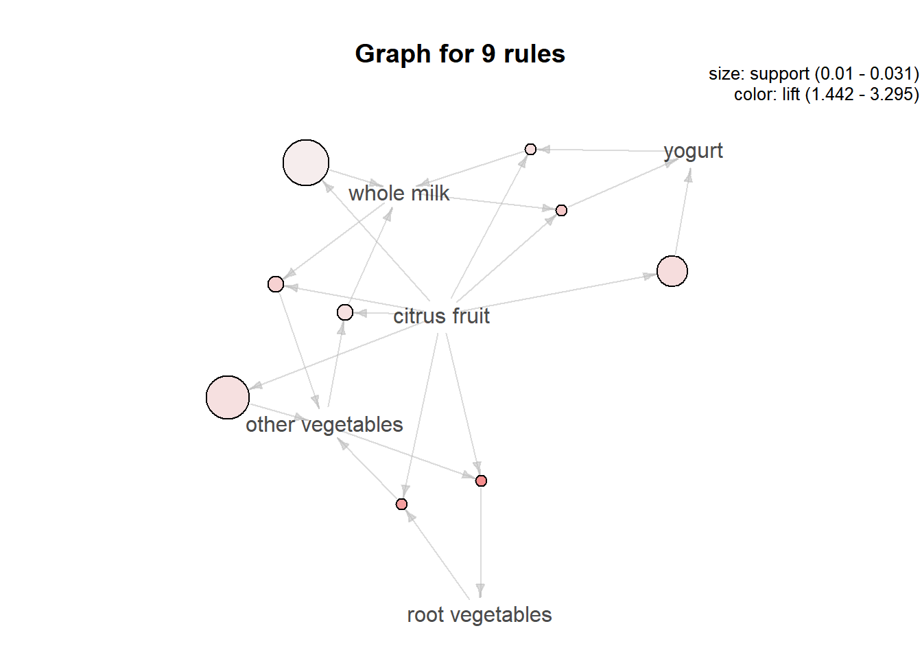
We can also change the graph layout.
plot(citrus.rules, method="graph", control=list(layout=igraph::in_circle()))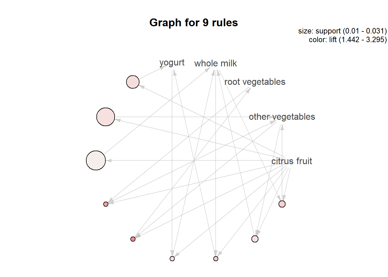
We can represent the rules as a grouped matrix-based visualization. The support and lift measures are represented by the size and color of the balloons, respectively.
plot(citrus.rules, method="grouped")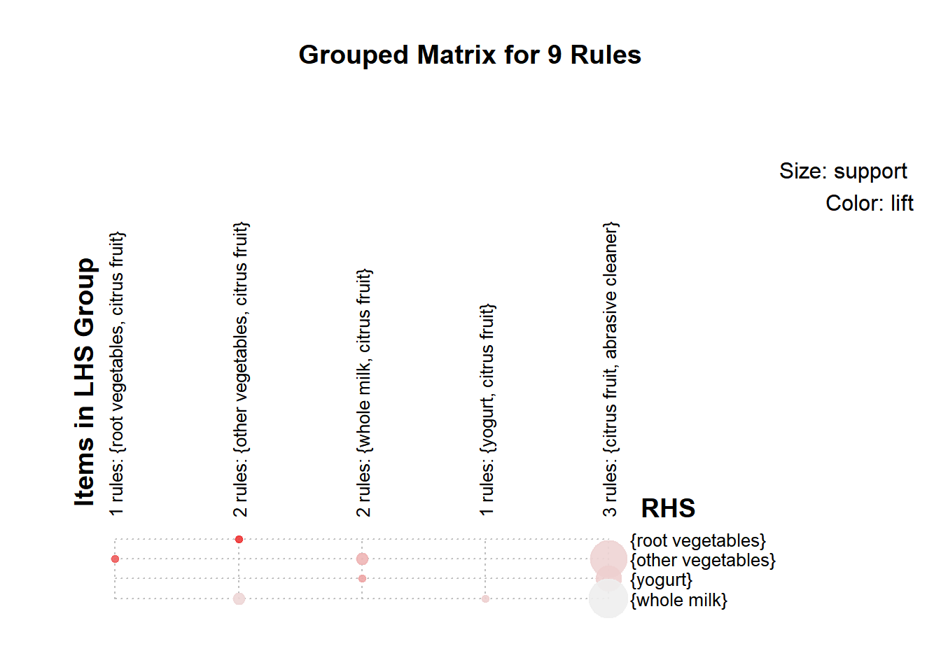
We can also use a parallel coordinates plot.
plot(citrus.rules, method="paracoord", control=list(reorder=TRUE))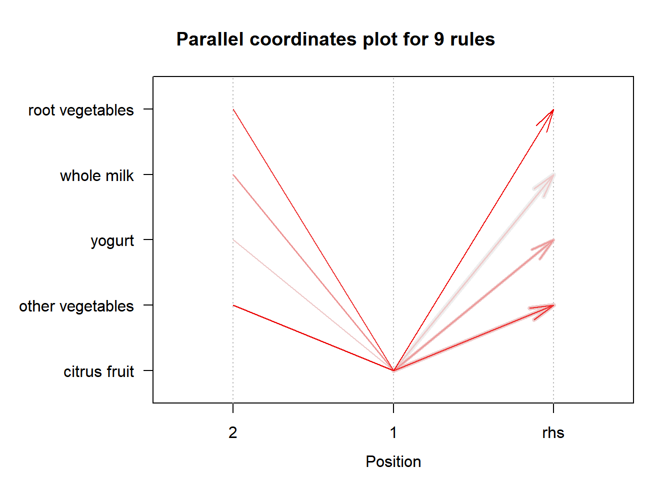
The function ruleExplorer() can explore association rules interactively.
10.5 References
- https://www.kaggle.com/xvivancos/market-basket-analysis
- Michael Hahsler, Kurt Hornik, and Thomas Reutterer (2006) Implications of probabilistic data modeling for mining association rules. In M. Spiliopoulou, R. Kruse, C. Borgelt, A. Nuernberger, and W. Gaul, editors, From Data and Information Analysis to Knowledge Engineering, Studies in Classification, Data Analysis, and Knowledge Organization, pages 598–605. Springer-Verlag.
- Michael Hahsler, Christian Buchta, Bettina Gruen and Kurt Hornik (2018). arules: Mining Association Rules and Frequent Itemsets. R package version 1.6-1. https://CRAN.R-project.org/package=arules
- Michael Hahsler, Bettina Gruen and Kurt Hornik (2005), arules - A Computational Environment for Mining Association Rules and Frequent Item Sets. Journal of Statistical Software 14/15. URL: http://dx.doi.org/10.18637/jss.v014.i15.
- Michael Hahsler, Sudheer Chelluboina, Kurt Hornik, and Christian Buchta (2011), The arules R-package ecosystem: Analyzing interesting patterns from large transaction datasets. Journal of Machine Learning Research, 12:1977–1981. URL: http://jmlr.csail.mit.edu/papers/v12/hahsler11a.html.
- Michael Hahsler (2018). arulesViz: Visualizing Association Rules and Frequent Itemsets. R package version 1.3-1. https://CRAN.R-project.org/package=arulesViz