Chapter 3 Data Manipulation
Data manipulation, data pre-procession, data organization, or data transformation is probably the most critical and challenging part of statistical data analysis. In this class, we will learn different ways to process data.
3.1 Data
We will use data collected in a study to show how to process typical data.
3.1.1 Background of the study
Recruitment of participants was conducted through four universities: a private university in the West, a private university in the Midwest, and public university in the East, and a public university in the South. Each university granted IRB approval for conducting the study. Participants were recruited through the psychology department subject pools at each university, as well as flyers posted on department bulletin boards.
In all cases, individuals were directed to a sign-up webpage. This page was an online consent form that included the details of the study as well as buttons they were to click to indicate their willingness to participate. Those who agreed to participate were then taken to a page where they provided their contact information (including an email address). Email addresses for those enrolled in the study were imported into Qualtrics, the software program used for designing and distributing the survey.
A few days after enrolling in the study, participants were sent an email that included a link to a baseline survey. This survey included a number of demographic questions as well as a series of trait measures of variables of interest to the research team. Then, a few days after that participants started receiving an email every day with a link to a daily survey that included a series of state measures pertaining to “this last day.” They received these daily emails for the next 50 days, with each daily survey being identical in nature. These daily survey links were sent in the evenings, and each link was only good for 24 hours.
Compensation was provided in three different ways. For completing the baseline survey participants who were currently enrolled in psychology courses received extra credit. Participants were also compensated based on the number of daily surveys they completed. They were paid 1 dollar per day for the first 20 daily surveys completed, 2 dollars per day for the next 20, and 3 dollars per day for the last 10 (in other words, there was a total of 90 dollars possible if they completed all 50 surveys). Lastly, 10 Amazon.com gift certificates of 100 dollars each were awarded through a raffle. Individuals received one raffle ticket for each 10 surveys they completed (these did not need to be consecutive). To conduct the raffle, participant ID numbers were entered into a random number generator (one time for each ticket received).
3.1.2 Measures
All of the measures for the present study were self-reported and were completed on a daily basis for 50 days depending on the individual completion rate). Each measure asked participants to report on their behaviors, thoughts, or emotions during the “last day.”
3.1.2.1 Daily religious activities.
Respondents were first presented a web page with a list of 16 religious activities (e.g., “prayed,” “attended religious worship services,” and “studied scriptures individually”) and asked to select the activities they had participated in during the last day. Next, they were presented separate web pages for each of the selected activities and asked to do the following: “(1) Indicate the approximate number of minutes you spent in this activity over the last day. (2) Rate the quality of your time spent in this activity during the last day. In other words, indicate the average value, significance, or impact of the time spent in this activity on the scale from ‘not at all valuable’ to ‘extremely valuable’.” For the minutes involved in the activity, participants entered a number in a cell provided. The quality of the time spent on that activity during the last day was assessed using a slider with response labels.
3.1.2.2 Daily spiritual experiences.
Respondents were first presented a web page with a list of 18 spiritual experiences (e.g., “I felt guided by God or the Spirit of God,” “I felt comfort, calm release, or peace,” and “I sensed an increase in emotional or spiritual strength”) and asked to select those they had experienced in during the last day. Next, they were presented separate web pages for each of the selected experiences and asked to do the following: “(1) Record how often you had this type of experience during the last day. (2) Rate the quality of those experiences. Indicate the average intensity, depth, quality, or significance of this type of experience during the last day on the scale from ‘not at all significant’ to ‘extremely significant’.” Participants indicated the frequency of spiritual experiences for a given day on a 5-point scale from “not at all” to “very often or most of the day.” The quality of the spiritual experiences during the last day was assessed using a slider with response labels.
3.1.2.3 Daily moral affect.
The moral emotions of empathy, gratitude, and forgiveness were assessed on a daily basis using 9 items (three for each emotion). Based on the procedures for the Positive and Negative Affect Schedule (Watson & Clark, 1994), we asked participants to “Indicate to what extent you felt the emotion during the last day on average on a scale from ‘not at all’ to ‘extremely’.” The three items for each emotion were derived from prior research on empathy (sympathetic, softhearted, and compassionate; Batson, Lishner, Cook, & Sawyer, 2005), gratitude (grateful, thankful, appreciative; Emmons & Kneezel, 2005) and forgiveness (hateful, resentful, forgiving; McCullough et al., 1998).
3.1.3 Data files
The baseline data and daily data are saved in two separated files. The original data were in SPSS format. I saved them into csv files from within SPSS.
- Baseline data: relig-baseline.csv
- Daily data: relig-daily.csv
3.2 Basic data information
As learned in the previous classes, we can use read.csv or read_csv to load data. Here, we use read_csv from the package readr. To load the package, we simply load tidyverse.
library(tidyverse)

baseline <- read_csv('data/relig-baseline.csv')

baseline
## # A tibble: 138 x 373
##    code     id start               end                 finish   age   sex
##    <chr> <dbl> <dttm>              <dttm>               <dbl> <dbl> <dbl>
##  1 R_25~   120 2009-10-08 09:44:14 2009-10-08 10:03:50      0    38     1
##  2 R_3O~   194 2009-10-05 15:49:36 2009-10-05 16:09:58      1    18     2
##  3 R_1M~   173 2009-10-05 16:05:44 2009-10-05 17:28:34      1    18     2
##  4 R_bC~   225 2009-10-05 12:55:48 2009-10-05 13:15:21      1    22     2
##  5 R_8n~   185 2009-10-05 12:59:46 2009-10-05 13:24:21      1    21     2
##  6 R_4H~   137 2009-10-05 13:01:37 2009-10-05 13:30:31      1    61     2
##  7 R_24~   164 2009-10-05 12:55:05 2009-10-05 13:13:52      1    25     2
##  8 R_01~   218 2009-10-05 20:29:52 2009-10-05 20:52:08      1    20     2
##  9 R_ai~   186 2009-10-05 15:01:44 2009-10-05 15:26:35      1    18     1
## 10 R_6X~   199 2009-10-05 13:32:58 2009-10-05 13:52:44      1    22     2
## # ... with 128 more rows, and 366 more variables: ethnicity <dbl>,
## #   ethnicityother <chr>, religaff <dbl>, religaff2 <dbl>, religaffother <chr>,
## #   relafa <dbl>, relafb <dbl>, relafc <dbl>, relafd <dbl>, marital <dbl>,
## #   maritalother <lgl>, edulevel <dbl>, edustatus <dbl>, edustatusother <chr>,
## #   incomeoption <dbl>, income <dbl>, depress1 <dbl>, depress2 <dbl>,
## #   depress3 <dbl>, depress4 <dbl>, depress5 <dbl>, depress6 <dbl>,
## #   depress7 <dbl>, depress8 <dbl>, depress9 <dbl>, depress10 <dbl>,
## #   depress11 <dbl>, depress12 <dbl>, depress13 <dbl>, depress14 <dbl>,
## #   depress15 <dbl>, depress16 <dbl>, depress17 <dbl>, depress18 <dbl>,
## #   depress19 <dbl>, depress20 <dbl>, depress21 <dbl>, parent1 <dbl>,
## #   parent2 <dbl>, parent3 <dbl>, parent4 <dbl>, parent5 <dbl>, parent6 <dbl>,
## #   parent7 <dbl>, parent8 <dbl>, parent9 <dbl>, parent10 <dbl>,
## #   parent11 <dbl>, parent12 <dbl>, parent13 <dbl>, parent14 <dbl>,
## #   parent15 <dbl>, parent16 <dbl>, parent17 <dbl>, parent18 <dbl>,
## #   parent19 <dbl>, parent20 <dbl>, parent21 <dbl>, parent22 <dbl>,
## #   parent23 <dbl>, parent24 <dbl>, parent25 <dbl>, parent26 <dbl>,
## #   parent27 <dbl>, parent28r <dbl>, parent29 <dbl>, parent30 <dbl>,
## #   person1 <dbl>, person2r <dbl>, person3 <dbl>, person4r <dbl>,
## #   person5 <dbl>, person6r <dbl>, person7 <dbl>, person8r <dbl>,
## #   person9 <dbl>, person10r <dbl>, ident1 <dbl>, ident2 <dbl>, ident3 <dbl>,
## #   ident4 <dbl>, ident5 <dbl>, ident6 <dbl>, ident7 <dbl>, ident8 <dbl>,
## #   ident9 <dbl>, ident10 <dbl>, ident11 <dbl>, ident12 <dbl>, ident13 <dbl>,
## #   ident14 <dbl>, ident15 <dbl>, ident16 <dbl>, ident17 <dbl>, ident18 <dbl>,
## #   ident19 <dbl>, ident20 <dbl>, ident21 <dbl>, ident22 <dbl>, ident23 <dbl>,
## #   ...
We can see there are nrow(baseline) participants and ncol(baseline) variables in the data file. The data are in the tibble format. When printing a tibble, only part of the data is shown to avoid to crowd the screen.
To get more detailed information about a data set, we can use the str() function.
str(baseline)3.3 Subsetting data
We first see how to select a subset of data.
3.3.1 Select columns (variables)
The base R typically uses two ways to select a subset of variables: using the numerical index or variable names. Suppose we are only interested in getting several demographic variables: age, sex, and level of education (edulevel).
In an R data set, each variable is numbered from 1 to P (the total number of variables). If we know the index, we can get them directly.
baseline[, c(6,7,19)]
## # A tibble: 138 x 3
##      age   sex edulevel
##    <dbl> <dbl>    <dbl>
##  1    38     1        6
##  2    18     2        2
##  3    18     2        3
##  4    22     2        3
##  5    21     2        3
##  6    61     2        7
##  7    25     2        7
##  8    20     2        3
##  9    18     1        3
## 10    22     2        3
## # ... with 128 more rows
Many times, using the variable names is more intuitive.
baseline[, c("age","sex","edulevel")]
## # A tibble: 138 x 3
##      age   sex edulevel
##    <dbl> <dbl>    <dbl>
##  1    38     1        6
##  2    18     2        2
##  3    18     2        3
##  4    22     2        3
##  5    21     2        3
##  6    61     2        7
##  7    25     2        7
##  8    20     2        3
##  9    18     1        3
## 10    22     2        3
## # ... with 128 more rows
The select function of the dplyr provides more ways to select a subset of variables.
select(baseline, age, sex, edulevel)
## # A tibble: 138 x 3
##      age   sex edulevel
##    <dbl> <dbl>    <dbl>
##  1    38     1        6
##  2    18     2        2
##  3    18     2        3
##  4    22     2        3
##  5    21     2        3
##  6    61     2        7
##  7    25     2        7
##  8    20     2        3
##  9    18     1        3
## 10    22     2        3
## # ... with 128 more rows
dplyr also provides a new operation in order to simplify the data processing. The operation is “%>%” from the R package magrittr. The %>% is called “pipe” which is added at the end of the code to tell R to keep receiving new commands.
Suppose x is a data set and we need to apply a function to f to x. In the base R way, we have f(x). Using ‘pipe’ method, we write it as x %>% f instead. If additional information is needed such as f(x,y), then we use x %>% f(y).
For the same example, we have:
baseline %>%
         select(age, sex, edulevel)
## # A tibble: 138 x 3
##      age   sex edulevel
##    <dbl> <dbl>    <dbl>
##  1    38     1        6
##  2    18     2        2
##  3    18     2        3
##  4    22     2        3
##  5    21     2        3
##  6    61     2        7
##  7    25     2        7
##  8    20     2        3
##  9    18     1        3
## 10    22     2        3
## # ... with 128 more rows
select can do much more than the basic usage here. For example, the data set has 21 depression variables named depress1 to depress21. To select all the variables, we use
baseline %>% select(age:edulevel)
## # A tibble: 138 x 14
##      age   sex ethnicity ethnicityother religaff religaff2 religaffother relafa
##    <dbl> <dbl>     <dbl> <chr>             <dbl>     <dbl> <chr>          <dbl>
##  1    38     1         2 <NA>                  1         1 <NA>               1
##  2    18     2         1 <NA>                  1         1 <NA>               1
##  3    18     2         1 <NA>                  1         1 <NA>               1
##  4    22     2         1 <NA>                  1         1 <NA>               1
##  5    21     2         1 <NA>                  1         1 <NA>               1
##  6    61     2         1 <NA>                  1         1 <NA>               1
##  7    25     2         7 Asian                 1         1 <NA>               1
##  8    20     2         1 <NA>                  1         1 <NA>               1
##  9    18     1         1 <NA>                  1         1 <NA>               1
## 10    22     2         1 <NA>                  1         1 <NA>               1
## # ... with 128 more rows, and 6 more variables: relafb <dbl>, relafc <dbl>,
## #   relafd <dbl>, marital <dbl>, maritalother <lgl>, edulevel <dbl>

baseline %>% select(depress1:depress21)
## # A tibble: 138 x 21
##    depress1 depress2 depress3 depress4 depress5 depress6 depress7 depress8
##       <dbl>    <dbl>    <dbl>    <dbl>    <dbl>    <dbl>    <dbl>    <dbl>
##  1        2        2        1        2        2        1        2        2
##  2        0        0        0        0        0        0        0        3
##  3        0        1        0        0        0        0        0        1
##  4        0        0        1        0        0        0        0        0
##  5        0        0        0        0        0        0        0        2
##  6        0        0        0        0        0        0        0        0
##  7        0        0        0        0        0        0        0        0
##  8        1        1        1        1        1        0        0        0
##  9        0        0        1        0        0        0        0        2
## 10        0        0        1        0        0        0        0        1
## # ... with 128 more rows, and 13 more variables: depress9 <dbl>,
## #   depress10 <dbl>, depress11 <dbl>, depress12 <dbl>, depress13 <dbl>,
## #   depress14 <dbl>, depress15 <dbl>, depress16 <dbl>, depress17 <dbl>,
## #   depress18 <dbl>, depress19 <dbl>, depress20 <dbl>, depress21 <dbl>
Here, A:B will select all the variables from A to B.
We can also remove variables in the following way. Using “-”, we remove variables from the data set.
baseline %>% select(-(code:income), -(parent1:negaff))
## # A tibble: 138 x 21
##    depress1 depress2 depress3 depress4 depress5 depress6 depress7 depress8
##       <dbl>    <dbl>    <dbl>    <dbl>    <dbl>    <dbl>    <dbl>    <dbl>
##  1        2        2        1        2        2        1        2        2
##  2        0        0        0        0        0        0        0        3
##  3        0        1        0        0        0        0        0        1
##  4        0        0        1        0        0        0        0        0
##  5        0        0        0        0        0        0        0        2
##  6        0        0        0        0        0        0        0        0
##  7        0        0        0        0        0        0        0        0
##  8        1        1        1        1        1        0        0        0
##  9        0        0        1        0        0        0        0        2
## 10        0        0        1        0        0        0        0        1
## # ... with 128 more rows, and 13 more variables: depress9 <dbl>,
## #   depress10 <dbl>, depress11 <dbl>, depress12 <dbl>, depress13 <dbl>,
## #   depress14 <dbl>, depress15 <dbl>, depress16 <dbl>, depress17 <dbl>,
## #   depress18 <dbl>, depress19 <dbl>, depress20 <dbl>, depress21 <dbl>
Functions can also be used in select(). The following functions are useful.
num_range("x", 1:3): matches x1, x2 and x3.starts_with("abc"): matches names that begin with “abc”.ends_with("xyz"): matches names that end with “xyz”.contains("ijk"): matches names that contain “ijk”.
baseline %>% select(num_range('depress', 1:21))
## # A tibble: 138 x 21
##    depress1 depress2 depress3 depress4 depress5 depress6 depress7 depress8
##       <dbl>    <dbl>    <dbl>    <dbl>    <dbl>    <dbl>    <dbl>    <dbl>
##  1        2        2        1        2        2        1        2        2
##  2        0        0        0        0        0        0        0        3
##  3        0        1        0        0        0        0        0        1
##  4        0        0        1        0        0        0        0        0
##  5        0        0        0        0        0        0        0        2
##  6        0        0        0        0        0        0        0        0
##  7        0        0        0        0        0        0        0        0
##  8        1        1        1        1        1        0        0        0
##  9        0        0        1        0        0        0        0        2
## 10        0        0        1        0        0        0        0        1
## # ... with 128 more rows, and 13 more variables: depress9 <dbl>,
## #   depress10 <dbl>, depress11 <dbl>, depress12 <dbl>, depress13 <dbl>,
## #   depress14 <dbl>, depress15 <dbl>, depress16 <dbl>, depress17 <dbl>,
## #   depress18 <dbl>, depress19 <dbl>, depress20 <dbl>, depress21 <dbl>

baseline %>% select(starts_with('depress'))
## # A tibble: 138 x 21
##    depress1 depress2 depress3 depress4 depress5 depress6 depress7 depress8
##       <dbl>    <dbl>    <dbl>    <dbl>    <dbl>    <dbl>    <dbl>    <dbl>
##  1        2        2        1        2        2        1        2        2
##  2        0        0        0        0        0        0        0        3
##  3        0        1        0        0        0        0        0        1
##  4        0        0        1        0        0        0        0        0
##  5        0        0        0        0        0        0        0        2
##  6        0        0        0        0        0        0        0        0
##  7        0        0        0        0        0        0        0        0
##  8        1        1        1        1        1        0        0        0
##  9        0        0        1        0        0        0        0        2
## 10        0        0        1        0        0        0        0        1
## # ... with 128 more rows, and 13 more variables: depress9 <dbl>,
## #   depress10 <dbl>, depress11 <dbl>, depress12 <dbl>, depress13 <dbl>,
## #   depress14 <dbl>, depress15 <dbl>, depress16 <dbl>, depress17 <dbl>,
## #   depress18 <dbl>, depress19 <dbl>, depress20 <dbl>, depress21 <dbl>

baseline %>% select(contains('depress'))
## # A tibble: 138 x 21
##    depress1 depress2 depress3 depress4 depress5 depress6 depress7 depress8
##       <dbl>    <dbl>    <dbl>    <dbl>    <dbl>    <dbl>    <dbl>    <dbl>
##  1        2        2        1        2        2        1        2        2
##  2        0        0        0        0        0        0        0        3
##  3        0        1        0        0        0        0        0        1
##  4        0        0        1        0        0        0        0        0
##  5        0        0        0        0        0        0        0        2
##  6        0        0        0        0        0        0        0        0
##  7        0        0        0        0        0        0        0        0
##  8        1        1        1        1        1        0        0        0
##  9        0        0        1        0        0        0        0        2
## 10        0        0        1        0        0        0        0        1
## # ... with 128 more rows, and 13 more variables: depress9 <dbl>,
## #   depress10 <dbl>, depress11 <dbl>, depress12 <dbl>, depress13 <dbl>,
## #   depress14 <dbl>, depress15 <dbl>, depress16 <dbl>, depress17 <dbl>,
## #   depress18 <dbl>, depress19 <dbl>, depress20 <dbl>, depress21 <dbl>
select() can be used together with everything() to move some variables to the start of a data frame.
baseline %>% select(age, sex, edulevel, everything())
## # A tibble: 138 x 373
##      age   sex edulevel code     id start               end
##    <dbl> <dbl>    <dbl> <chr> <dbl> <dttm>              <dttm>
##  1    38     1        6 R_25~   120 2009-10-08 09:44:14 2009-10-08 10:03:50
##  2    18     2        2 R_3O~   194 2009-10-05 15:49:36 2009-10-05 16:09:58
##  3    18     2        3 R_1M~   173 2009-10-05 16:05:44 2009-10-05 17:28:34
##  4    22     2        3 R_bC~   225 2009-10-05 12:55:48 2009-10-05 13:15:21
##  5    21     2        3 R_8n~   185 2009-10-05 12:59:46 2009-10-05 13:24:21
##  6    61     2        7 R_4H~   137 2009-10-05 13:01:37 2009-10-05 13:30:31
##  7    25     2        7 R_24~   164 2009-10-05 12:55:05 2009-10-05 13:13:52
##  8    20     2        3 R_01~   218 2009-10-05 20:29:52 2009-10-05 20:52:08
##  9    18     1        3 R_ai~   186 2009-10-05 15:01:44 2009-10-05 15:26:35
## 10    22     2        3 R_6X~   199 2009-10-05 13:32:58 2009-10-05 13:52:44
## # ... with 128 more rows, and 366 more variables: finish <dbl>,
## #   ethnicity <dbl>, ethnicityother <chr>, religaff <dbl>, religaff2 <dbl>,
## #   religaffother <chr>, relafa <dbl>, relafb <dbl>, relafc <dbl>,
## #   relafd <dbl>, marital <dbl>, maritalother <lgl>, edustatus <dbl>,
## #   edustatusother <chr>, incomeoption <dbl>, income <dbl>, depress1 <dbl>,
## #   depress2 <dbl>, depress3 <dbl>, depress4 <dbl>, depress5 <dbl>,
## #   depress6 <dbl>, depress7 <dbl>, depress8 <dbl>, depress9 <dbl>,
## #   depress10 <dbl>, depress11 <dbl>, depress12 <dbl>, depress13 <dbl>,
## #   depress14 <dbl>, depress15 <dbl>, depress16 <dbl>, depress17 <dbl>,
## #   depress18 <dbl>, depress19 <dbl>, depress20 <dbl>, depress21 <dbl>,
## #   parent1 <dbl>, parent2 <dbl>, parent3 <dbl>, parent4 <dbl>, parent5 <dbl>,
## #   parent6 <dbl>, parent7 <dbl>, parent8 <dbl>, parent9 <dbl>, parent10 <dbl>,
## #   parent11 <dbl>, parent12 <dbl>, parent13 <dbl>, parent14 <dbl>,
## #   parent15 <dbl>, parent16 <dbl>, parent17 <dbl>, parent18 <dbl>,
## #   parent19 <dbl>, parent20 <dbl>, parent21 <dbl>, parent22 <dbl>,
## #   parent23 <dbl>, parent24 <dbl>, parent25 <dbl>, parent26 <dbl>,
## #   parent27 <dbl>, parent28r <dbl>, parent29 <dbl>, parent30 <dbl>,
## #   person1 <dbl>, person2r <dbl>, person3 <dbl>, person4r <dbl>,
## #   person5 <dbl>, person6r <dbl>, person7 <dbl>, person8r <dbl>,
## #   person9 <dbl>, person10r <dbl>, ident1 <dbl>, ident2 <dbl>, ident3 <dbl>,
## #   ident4 <dbl>, ident5 <dbl>, ident6 <dbl>, ident7 <dbl>, ident8 <dbl>,
## #   ident9 <dbl>, ident10 <dbl>, ident11 <dbl>, ident12 <dbl>, ident13 <dbl>,
## #   ident14 <dbl>, ident15 <dbl>, ident16 <dbl>, ident17 <dbl>, ident18 <dbl>,
## #   ident19 <dbl>, ident20 <dbl>, ident21 <dbl>, ident22 <dbl>, ident23 <dbl>,
## #   ...
3.3.2 Select rows (participants)
The religious data set has a variable sex with 1 denoting male and 2 denoting female. Suppose we want to take out male data.
The R base method is
baseline[baseline$sex == 1, c('age','edulevel')]
## # A tibble: 25 x 2
##      age edulevel
##    <dbl>    <dbl>
##  1    38        6
##  2    18        3
##  3    31        3
##  4    57        2
##  5    23        5
##  6    21        3
##  7    22        3
##  8    22        3
##  9    15        1
## 10    21        2
## # ... with 15 more rows
The filter() function of the package dplyr provides more options for selecting a subset of data.
baseline %>%
  select(age, sex, edulevel) %>%
  filter(sex==1)
## # A tibble: 25 x 3
##      age   sex edulevel
##    <dbl> <dbl>    <dbl>
##  1    38     1        6
##  2    18     1        3
##  3    31     1        3
##  4    57     1        2
##  5    23     1        5
##  6    21     1        3
##  7    22     1        3
##  8    22     1        3
##  9    15     1        1
## 10    21     1        2
## # ... with 15 more rows

baseline %>%
  filter(sex==1)%>%
  select(age, sex, edulevel)
## # A tibble: 25 x 3
##      age   sex edulevel
##    <dbl> <dbl>    <dbl>
##  1    38     1        6
##  2    18     1        3
##  3    31     1        3
##  4    57     1        2
##  5    23     1        5
##  6    21     1        3
##  7    22     1        3
##  8    22     1        3
##  9    15     1        1
## 10    21     1        2
## # ... with 15 more rows
Using two variables for selection
baseline %>%
  select(age, sex, edulevel) %>%
  filter(age < 21, sex==2)
## # A tibble: 58 x 3
##      age   sex edulevel
##    <dbl> <dbl>    <dbl>
##  1    18     2        2
##  2    18     2        3
##  3    20     2        3
##  4    20     2        3
##  5    20     2        3
##  6    18     2        3
##  7    20     2        3
##  8    18     2        2
##  9    19     2        3
## 10    19     2        3
## # ... with 48 more rows
3.4 Rearrange data
3.4.1 Order data
The function arrange() can be used to sort data. By default, it sorts data in the ascending order.
baseline %>%
  select(age, sex, edulevel) %>%
  arrange(age)
## # A tibble: 138 x 3
##      age   sex edulevel
##    <dbl> <dbl>    <dbl>
##  1    13     2        1
##  2    15     1        1
##  3    17     2        3
##  4    18     2        2
##  5    18     2        3
##  6    18     1        3
##  7    18     2        3
##  8    18     2        2
##  9    18     1        2
## 10    18     2        2
## # ... with 128 more rows
To change to the descending order, use
baseline %>%
  select(age, sex, edulevel) %>%
  arrange(desc(age))
## # A tibble: 138 x 3
##      age   sex edulevel
##    <dbl> <dbl>    <dbl>
##  1    69     2        3
##  2    61     2        7
##  3    57     1        2
##  4    54     2        6
##  5    54     2        3
##  6    53     2        5
##  7    53     2        4
##  8    48     2        7
##  9    48     2        3
## 10    41     2        3
## # ... with 128 more rows
Sorting based on two or more variables
baseline %>%
  select(age, sex, edulevel) %>%
  arrange(sex, edulevel, age) %>%
  select(sex, edulevel, age)
## # A tibble: 138 x 3
##      sex edulevel   age
##    <dbl>    <dbl> <dbl>
##  1     1        1    15
##  2     1        2    18
##  3     1        2    21
##  4     1        2    24
##  5     1        2    57
##  6     1        3    18
##  7     1        3    18
##  8     1        3    20
##  9     1        3    21
## 10     1        3    21
## # ... with 128 more rows
3.4.2 Add new rows
R is not for data management. So in general, it is not recommended to directly add new rows of data to the existing data frame. But for simple data addition, it is possible and easy. Here, we use the function add_row to do the work. For demonstration, we first select a subset of data.
subset.base <- baseline %>%
                select(age, sex, edulevel)

subset.base
## # A tibble: 138 x 3
##      age   sex edulevel
##    <dbl> <dbl>    <dbl>
##  1    38     1        6
##  2    18     2        2
##  3    18     2        3
##  4    22     2        3
##  5    21     2        3
##  6    61     2        7
##  7    25     2        7
##  8    20     2        3
##  9    18     1        3
## 10    22     2        3
## # ... with 128 more rows
Now, suppose we forgot to include data from a participant with age = 20, sex = 1, and edulevel =5.
- Add the data at the end
subset.base %>%
            add_row(age = 20, sex = 1, edulevel =5) %>%
            tail()
## # A tibble: 6 x 3
##     age   sex edulevel
##   <dbl> <dbl>    <dbl>
## 1    19     2        3
## 2    20     2        3
## 3    20     2        2
## 4    22     1        3
## 5    20     1        3
## 6 20 1 5- Add to the beginning of the data set
subset.base %>%
            add_row(age = 20, sex = 1,
                    edulevel = 5, .before = 1)
## # A tibble: 139 x 3
##      age   sex edulevel
##    <dbl> <dbl>    <dbl>
##  1    20     1        5
##  2    38     1        6
##  3    18     2        2
##  4    18     2        3
##  5    22     2        3
##  6    21     2        3
##  7    61     2        7
##  8    25     2        7
##  9    20     2        3
## 10    18     1        3
## # ... with 129 more rows- Use the function
rbind.
subset.base %>%
            rbind(c(20, 1, 5))
## # A tibble: 139 x 3
##      age   sex edulevel
##    <dbl> <dbl>    <dbl>
##  1    38     1        6
##  2    18     2        2
##  3    18     2        3
##  4    22     2        3
##  5    21     2        3
##  6    61     2        7
##  7    25     2        7
##  8    20     2        3
##  9    18     1        3
## 10    22     2        3
## # ... with 129 more rows- Add calculated values: the average of age and edulevel.
.replaces it with the one on the left-hand side of%>%.
subset.base %>%
            add_row(age = mean(.$age),
                    edulevel = mean(.$edulevel),
                    .before = 1)
## # A tibble: 139 x 3
##      age   sex edulevel
##    <dbl> <dbl>    <dbl>
##  1  23.6    NA     3.16
##  2  38       1     6
##  3  18       2     2
##  4  18       2     3
##  5  22       2     3
##  6  21       2     3
##  7  61       2     7
##  8  25       2     7
##  9  20       2     3
## 10  18       1     3
## # ... with 129 more rows
3.4.3 Add new columns
Adding new columns to the existing data set is far more common. This is because we often create new variables based on the existing data. We show how to use the mutate() function.
- Add a new continuous id variable
subset.base %>%
  mutate(newid = 1:138) %>%
  select(newid, everything())
## # A tibble: 138 x 4
##    newid   age   sex edulevel
##    <int> <dbl> <dbl>    <dbl>
##  1     1    38     1        6
##  2     2    18     2        2
##  3     3    18     2        3
##  4     4    22     2        3
##  5     5    21     2        3
##  6     6    61     2        7
##  7     7    25     2        7
##  8     8    20     2        3
##  9     9    18     1        3
## 10    10    22     2        3
## # ... with 128 more rows- If a variable exists, its values will be replaced.
subset.base %>%
  mutate(newid = 1:138) %>%
  select(newid, everything()) %>%
  mutate(newid = nrow(.):1)
## # A tibble: 138 x 4
##    newid   age   sex edulevel
##    <int> <dbl> <dbl>    <dbl>
##  1   138    38     1        6
##  2   137    18     2        2
##  3   136    18     2        3
##  4   135    22     2        3
##  5   134    21     2        3
##  6   133    61     2        7
##  7   132    25     2        7
##  8   131    20     2        3
##  9   130    18     1        3
## 10   129    22     2        3
## # ... with 128 more rows

subset.base %>%
  mutate(newid = 1:138) %>%
  select(newid, everything()) %>%
  mutate(newid1 = nrow(.):1)
## # A tibble: 138 x 5
##    newid   age   sex edulevel newid1
##    <int> <dbl> <dbl>    <dbl>  <int>
##  1     1    38     1        6    138
##  2     2    18     2        2    137
##  3     3    18     2        3    136
##  4     4    22     2        3    135
##  5     5    21     2        3    134
##  6     6    61     2        7    133
##  7     7    25     2        7    132
##  8     8    20     2        3    131
##  9     9    18     1        3    130
## 10    10    22     2        3    129
## # ... with 128 more rows- Recode variables.
- Dummy code the sex variable to 0 and 1.
- Convert edulevel to three levels: no college (edulevel < 2), college (edulevel > 2 & <= 5), and gradaute (edulevel > 5).
subset.base %>%
            mutate(sex = sex -1, edu = case_when(
                  edulevel <=2 ~ 'no-college',
                  edulevel > 2 & edulevel <=5 ~ 'college',
                  edulevel > 5 ~ 'graduate'
                )
            )
## # A tibble: 138 x 4
##      age   sex edulevel edu
##    <dbl> <dbl>    <dbl> <chr>
##  1    38     0        6 graduate
##  2    18     1        2 no-college
##  3    18     1        3 college
##  4    22     1        3 college
##  5    21     1        3 college
##  6    61     1        7 graduate
##  7    25     1        7 graduate
##  8    20     1        3 college
##  9    18     0        3 college
## 10    22     1        3 college
## # ... with 128 more rows
Another way to do it.
subset.base %>%
            mutate(sex = sex - 1, edu = case_when(
                  edulevel <=2 ~ 'no-college',
                  edulevel > 5 ~ 'graduate',
                  TRUE ~ 'college',
                )
            )
## # A tibble: 138 x 4
##      age   sex edulevel edu
##    <dbl> <dbl>    <dbl> <chr>
##  1    38     0        6 graduate
##  2    18     1        2 no-college
##  3    18     1        3 college
##  4    22     1        3 college
##  5    21     1        3 college
##  6    61     1        7 graduate
##  7    25     1        7 graduate
##  8    20     1        3 college
##  9    18     0        3 college
## 10    22     1        3 college
## # ... with 128 more rows
subset.base %>%
mutate(age.cat = case_when(
age < 21 ~ 'g1',
age >= 21 ~ 'g2',
TRUE ~ 'NA'
)
)
## # A tibble: 138 x 4
## age sex edulevel age.cat
## <dbl> <dbl> <dbl> <chr>
## 1 38 1 6 g2
## 2 18 2 2 g1
## 3 18 2 3 g1
## 4 22 2 3 g2
## 5 21 2 3 g2
## 6 61 2 7 g2
## 7 25 2 7 g2
## 8 20 2 3 g1
## 9 18 1 3 g1
## 10 22 2 3 g2
## # ... with 128 more rowsA third way to do it
subset.base %>%
  mutate(sex = recode(sex, `1`='M', `2`='F'))
## # A tibble: 138 x 3
##      age sex   edulevel
##    <dbl> <chr>    <dbl>
##  1    38 M            6
##  2    18 F            2
##  3    18 F            3
##  4    22 F            3
##  5    21 F            3
##  6    61 F            7
##  7    25 F            7
##  8    20 F            3
##  9    18 M            3
## 10    22 F            3
## # ... with 128 more rows- Cut a variable into groups
The cut function of R base can be first used.
subset.base %>%
  mutate(sex = sex - 1,
        edu = cut(edulevel,
          c(min(edulevel),2,5,max(edulevel)),
          labels=c("no-college", "college", "graduate"))
        )
## # A tibble: 138 x 4
##      age   sex edulevel edu
##    <dbl> <dbl>    <dbl> <fct>
##  1    38     0        6 graduate
##  2    18     1        2 no-college
##  3    18     1        3 college
##  4    22     1        3 college
##  5    21     1        3 college
##  6    61     1        7 graduate
##  7    25     1        7 graduate
##  8    20     1        3 college
##  9    18     0        3 college
## 10    22     1        3 college
## # ... with 128 more rows
Sometimes, it is useful to create a numerical variable.
subset.base %>%
  mutate(sex = sex - 1,
        edu = cut(edulevel,
          c(min(edulevel),2,5,max(edulevel)),
          labels=1:3)
        ) %>%
  mutate(edu = as.numeric(edu))
## # A tibble: 138 x 4
##      age   sex edulevel   edu
##    <dbl> <dbl>    <dbl> <dbl>
##  1    38     0        6     3
##  2    18     1        2     1
##  3    18     1        3     2
##  4    22     1        3     2
##  5    21     1        3     2
##  6    61     1        7     3
##  7    25     1        7     3
##  8    20     1        3     2
##  9    18     0        3     2
## 10    22     1        3     2
## # ... with 128 more rows
The R package ggplot2 has several functions to cut a variables - cut_interval makes n groups with equal range, cut_number makes n groups with (approximately) equal numbers of observations; cut_width makes groups of width width.
subset.base %>%
  mutate(
        age.interval = cut_interval(age, 3),
        age.number = cut_number(age, 3),
        age.width = cut_width(age, 5)
        )
## # A tibble: 138 x 6
##      age   sex edulevel age.interval age.number age.width
##    <dbl> <dbl>    <dbl> <fct>        <fct>      <fct>
##  1    38     1        6 (31.7,50.3]  (21,69]    (37.5,42.5]
##  2    18     2        2 [13,31.7]    [13,20]    (17.5,22.5]
##  3    18     2        3 [13,31.7]    [13,20]    (17.5,22.5]
##  4    22     2        3 [13,31.7]    (21,69]    (17.5,22.5]
##  5    21     2        3 [13,31.7]    (20,21]    (17.5,22.5]
##  6    61     2        7 (50.3,69]    (21,69]    (57.5,62.5]
##  7    25     2        7 [13,31.7]    (21,69]    (22.5,27.5]
##  8    20     2        3 [13,31.7]    [13,20]    (17.5,22.5]
##  9    18     1        3 [13,31.7]    [13,20]    (17.5,22.5]
## 10    22     2        3 [13,31.7]    (21,69]    (17.5,22.5]
## # ... with 128 more rows
subset.base %>%
mutate(
age.interval = cut_interval(age, 3),
age.number = cut_number(age, 3),
age.width = cut_width(age, 5)
) %>%
mutate(age.interval = as.numeric(age.interval),
age.number = as.numeric(age.interval),
age.width = as.numeric(age.width))
## # A tibble: 138 x 6
## age sex edulevel age.interval age.number age.width
## <dbl> <dbl> <dbl> <dbl> <dbl> <dbl>
## 1 38 1 6 2 2 6
## 2 18 2 2 1 1 2
## 3 18 2 3 1 1 2
## 4 22 2 3 1 1 2
## 5 21 2 3 1 1 2
## 6 61 2 7 3 3 10
## 7 25 2 7 1 1 3
## 8 20 2 3 1 1 2
## 9 18 1 3 1 1 2
## 10 22 2 3 1 1 2
## # ... with 128 more rows- Calculate the composite score of a depression test.
baseline %>%
  mutate(t.depress = select(., starts_with('depress')) %>% rowSums) %>%
  select(t.depress, everything())
## # A tibble: 138 x 374
##    t.depress code     id start               end                 finish   age
##        <dbl> <chr> <dbl> <dttm>              <dttm>               <dbl> <dbl>
##  1        31 R_25~   120 2009-10-08 09:44:14 2009-10-08 10:03:50      0    38
##  2        15 R_3O~   194 2009-10-05 15:49:36 2009-10-05 16:09:58      1    18
##  3         9 R_1M~   173 2009-10-05 16:05:44 2009-10-05 17:28:34      1    18
##  4         2 R_bC~   225 2009-10-05 12:55:48 2009-10-05 13:15:21      1    22
##  5         4 R_8n~   185 2009-10-05 12:59:46 2009-10-05 13:24:21      1    21
##  6         0 R_4H~   137 2009-10-05 13:01:37 2009-10-05 13:30:31      1    61
##  7         0 R_24~   164 2009-10-05 12:55:05 2009-10-05 13:13:52      1    25
##  8        14 R_01~   218 2009-10-05 20:29:52 2009-10-05 20:52:08      1    20
##  9        10 R_ai~   186 2009-10-05 15:01:44 2009-10-05 15:26:35      1    18
## 10         6 R_6X~   199 2009-10-05 13:32:58 2009-10-05 13:52:44      1    22
## # ... with 128 more rows, and 367 more variables: sex <dbl>, ethnicity <dbl>,
## #   ethnicityother <chr>, religaff <dbl>, religaff2 <dbl>, religaffother <chr>,
## #   relafa <dbl>, relafb <dbl>, relafc <dbl>, relafd <dbl>, marital <dbl>,
## #   maritalother <lgl>, edulevel <dbl>, edustatus <dbl>, edustatusother <chr>,
## #   incomeoption <dbl>, income <dbl>, depress1 <dbl>, depress2 <dbl>,
## #   depress3 <dbl>, depress4 <dbl>, depress5 <dbl>, depress6 <dbl>,
## #   depress7 <dbl>, depress8 <dbl>, depress9 <dbl>, depress10 <dbl>,
## #   depress11 <dbl>, depress12 <dbl>, depress13 <dbl>, depress14 <dbl>,
## #   depress15 <dbl>, depress16 <dbl>, depress17 <dbl>, depress18 <dbl>,
## #   depress19 <dbl>, depress20 <dbl>, depress21 <dbl>, parent1 <dbl>,
## #   parent2 <dbl>, parent3 <dbl>, parent4 <dbl>, parent5 <dbl>, parent6 <dbl>,
## #   parent7 <dbl>, parent8 <dbl>, parent9 <dbl>, parent10 <dbl>,
## #   parent11 <dbl>, parent12 <dbl>, parent13 <dbl>, parent14 <dbl>,
## #   parent15 <dbl>, parent16 <dbl>, parent17 <dbl>, parent18 <dbl>,
## #   parent19 <dbl>, parent20 <dbl>, parent21 <dbl>, parent22 <dbl>,
## #   parent23 <dbl>, parent24 <dbl>, parent25 <dbl>, parent26 <dbl>,
## #   parent27 <dbl>, parent28r <dbl>, parent29 <dbl>, parent30 <dbl>,
## #   person1 <dbl>, person2r <dbl>, person3 <dbl>, person4r <dbl>,
## #   person5 <dbl>, person6r <dbl>, person7 <dbl>, person8r <dbl>,
## #   person9 <dbl>, person10r <dbl>, ident1 <dbl>, ident2 <dbl>, ident3 <dbl>,
## #   ident4 <dbl>, ident5 <dbl>, ident6 <dbl>, ident7 <dbl>, ident8 <dbl>,
## #   ident9 <dbl>, ident10 <dbl>, ident11 <dbl>, ident12 <dbl>, ident13 <dbl>,
## #   ident14 <dbl>, ident15 <dbl>, ident16 <dbl>, ident17 <dbl>, ident18 <dbl>,
## #   ident19 <dbl>, ident20 <dbl>, ident21 <dbl>, ident22 <dbl>, ...

baseline %>%
  select(starts_with('depress')) %>%
  rowSums
##   [1] 31 15  9  2  4  0  0 14 10  6  8 17 32  2 14  4  3 15  3  5  4  8  6  3  6
##  [26] 14  5 11  0  0  5 NA  0  4  8  4 21  3  2  3 28 16  3  7  6  5 24 20  3  3
##  [51]  7 11 25  2 13  8 25  8  9  5  2  3  7 24  0  2  9  8 12 11 17  9  4 19  1
##  [76]  3  3  6  6 11  5  8 41  0  0 14  6  8 28  9  6 19  3 20 12  9 21  2  8  4
## [101] 21  1  4 NA  6  6 13  6  5  3  4 19 10  7  9 38 14  3  4  5  4  6 16  8  0
## [126] 26 13  0  2 18  7 50  4 13  5  9  2 12
Note that we can use only R base function to do the same job.
cbind(t.depress = apply(
  baseline[, paste0('depress', 1:21)], 1, sum),
  baseline)[1:10, 1:5]
##    t.depress              code  id               start                 end
## 1         31 R_25GIuwKLeewQwza 120 2009-10-08 09:44:14 2009-10-08 10:03:50
## 2         15 R_3OZklSb7cmTemmU 194 2009-10-05 15:49:36 2009-10-05 16:09:58
## 3          9 R_1M16fasJ5ToWsrq 173 2009-10-05 16:05:44 2009-10-05 17:28:34
## 4          2 R_bC8F2HhuZtHh0fW 225 2009-10-05 12:55:48 2009-10-05 13:15:21
## 5          4 R_8nXFYn8Hh0KSQN6 185 2009-10-05 12:59:46 2009-10-05 13:24:21
## 6          0 R_4HjdH4xZDR03Sdu 137 2009-10-05 13:01:37 2009-10-05 13:30:31
## 7          0 R_24rwrrQav6IL3SY 164 2009-10-05 12:55:05 2009-10-05 13:13:52
## 8         14 R_01dtSSOfCg38a2g 218 2009-10-05 20:29:52 2009-10-05 20:52:08
## 9         10 R_ai1lMellT5fi0rq 186 2009-10-05 15:01:44 2009-10-05 15:26:35
## 10 6 R_6XvgLEQJrUS7LDe 199 2009-10-05 13:32:58 2009-10-05 13:52:44- Only keep the new variables using the function
transmute.
baseline %>%
  transmute(t.depress = select(., starts_with('depress')) %>% rowSums)
## # A tibble: 138 x 1
##    t.depress
##        <dbl>
##  1        31
##  2        15
##  3         9
##  4         2
##  5         4
##  6         0
##  7         0
##  8        14
##  9        10
## 10         6
## # ... with 128 more rows
3.4.3.1 Practice
Using the baseline data, compare the average total emotion scores from male and female participants.
baseline %>%
  select(num_range('emo', 1:14), sex) %>%
  mutate(t.emotion = select(., starts_with('emo')) %>% rowSums) %>%
  select(sex, t.emotion) %>%
  filter(sex==1) %>%
  colMeans(na.rm=TRUE)
##       sex t.emotion
##     1.000    62.875

baseline %>%
  select(num_range('emo', 1:14), sex) %>%
  mutate(t.emotion = select(., starts_with('emo')) %>% rowSums) %>%
  select(sex, t.emotion) %>%
  filter(sex==2) %>%
  colMeans(na.rm=TRUE)
##       sex t.emotion
##   2.00000  62.75676


total.emo <- baseline %>%
  select(num_range('emo', 1:14), sex) %>%
  mutate(t.emotion = select(., starts_with('emo')) %>% rowSums) %>%
  select(sex, t.emotion) %>%
  filter(sex==2)

baseline %>%
  select(num_range('emo', 1:14), sex) %>%
  mutate(t.emotion = select(., starts_with('emo')) %>% rowSums) %>%
  select(sex, t.emotion) %>%
  filter(sex==2) -> temp

temp %>%
  mean(t.emotion, na.rm=TRUE)
## [1] NA
3.5 Grouping data
Most data operations are done on groups defined by variables. The function group_by() takes an existing data frame and converts it into a grouped data frame where operations are performed “by group”. The function ungroup() removes grouping.
- Group data based on sex
by.sex <- baseline %>%
      select(id, age, sex, edulevel,
             starts_with('depress')) %>%
      group_by(sex)

by.sex
## # A tibble: 138 x 25
## # Groups:   sex [2]
##       id   age   sex edulevel depress1 depress2 depress3 depress4 depress5
##    <dbl> <dbl> <dbl>    <dbl>    <dbl>    <dbl>    <dbl>    <dbl>    <dbl>
##  1   120    38     1        6        2        2        1        2        2
##  2   194    18     2        2        0        0        0        0        0
##  3   173    18     2        3        0        1        0        0        0
##  4   225    22     2        3        0        0        1        0        0
##  5   185    21     2        3        0        0        0        0        0
##  6   137    61     2        7        0        0        0        0        0
##  7   164    25     2        7        0        0        0        0        0
##  8   218    20     2        3        1        1        1        1        1
##  9   186    18     1        3        0        0        1        0        0
## 10   199    22     2        3        0        0        1        0        0
## # ... with 128 more rows, and 16 more variables: depress6 <dbl>,
## #   depress7 <dbl>, depress8 <dbl>, depress9 <dbl>, depress10 <dbl>,
## #   depress11 <dbl>, depress12 <dbl>, depress13 <dbl>, depress14 <dbl>,
## #   depress15 <dbl>, depress16 <dbl>, depress17 <dbl>, depress18 <dbl>,
## #   depress19 <dbl>, depress20 <dbl>, depress21 <dbl>
The grouped data are often used with the
summarizefunction.- For example, we get the sample size for each group.
by.sex %>% summarize(size = n())
## # A tibble: 2 x 2
##     sex  size
##   <dbl> <int>
## 1     1    25
## 2 2 113- Average age and education level
by.sex %>%
  summarize(m.age = mean(age),
            m.edu = mean(edulevel),
            size = n())
## # A tibble: 2 x 4
##     sex m.age m.edu  size
##   <dbl> <dbl> <dbl> <int>
## 1     1  24.7  3.2     25
## 2 2 23.3 3.15 113- More than one grouping variables
by.sex.edu <- baseline %>%
                  select(id, age, sex, edulevel,
                         starts_with('depress')) %>%
                  group_by(edulevel, sex)
by.sex.edu
## # A tibble: 138 x 25
## # Groups:   edulevel, sex [12]
##       id   age   sex edulevel depress1 depress2 depress3 depress4 depress5
##    <dbl> <dbl> <dbl>    <dbl>    <dbl>    <dbl>    <dbl>    <dbl>    <dbl>
##  1   120    38     1        6        2        2        1        2        2
##  2   194    18     2        2        0        0        0        0        0
##  3   173    18     2        3        0        1        0        0        0
##  4   225    22     2        3        0        0        1        0        0
##  5   185    21     2        3        0        0        0        0        0
##  6   137    61     2        7        0        0        0        0        0
##  7   164    25     2        7        0        0        0        0        0
##  8   218    20     2        3        1        1        1        1        1
##  9   186    18     1        3        0        0        1        0        0
## 10   199    22     2        3        0        0        1        0        0
## # ... with 128 more rows, and 16 more variables: depress6 <dbl>,
## #   depress7 <dbl>, depress8 <dbl>, depress9 <dbl>, depress10 <dbl>,
## #   depress11 <dbl>, depress12 <dbl>, depress13 <dbl>, depress14 <dbl>,
## #   depress15 <dbl>, depress16 <dbl>, depress17 <dbl>, depress18 <dbl>,
## # depress19 <dbl>, depress20 <dbl>, depress21 <dbl>- Mean age
by.sex.edu %>% summarize(m.age = mean(age))
## # A tibble: 12 x 3
## # Groups:   edulevel [7]
##    edulevel   sex m.age
##       <dbl> <dbl> <dbl>
##  1        1     1  15
##  2        1     2  13
##  3        2     1  30
##  4        2     2  19.4
##  5        3     1  22.1
##  6        3     2  21.9
##  7        4     2  31.5
##  8        5     1  23
##  9        5     2  36.4
## 10        6     1  35.7
## 11        6     2  33.7
## 12 7 2 44.7- Note that any function can be used here. But we need to make sure that the returned information conforms to the data format.
The R function lm() can be used to conduct a linear regression analysis. Suppose we want to get the regression slope between depression and age. We first write a function to get the coefficient.
slope <- function(y, x){
  model <- lm(y~x)
  coef(model)[2]
}
Then, we apply this function to the data.
by.sex.edu %>% ungroup() %>%
  mutate(t.depress = select(., starts_with('depress')) %>% rowSums) %>%
  group_by(sex, edulevel) %>%
   summarize(slope = slope(t.depress, age))
## # A tibble: 12 x 3
## # Groups:   sex [2]
##      sex edulevel    slope
##    <dbl>    <dbl>    <dbl>
##  1     1        1  NA
##  2     1        2  -0.139
##  3     1        3   0.334
##  4     1        5  NA
##  5     1        6   2.55
##  6     2        1  NA
##  7     2        2  -2.16
##  8     2        3   0.343
##  9     2        4  -0.394
## 10     2        5  -0.0326
## 11     2        6   0.191
## 12 2 7 0.0301- Ungroup data
by.sex.edu %>% ungroup()
## # A tibble: 138 x 25
##       id   age   sex edulevel depress1 depress2 depress3 depress4 depress5
##    <dbl> <dbl> <dbl>    <dbl>    <dbl>    <dbl>    <dbl>    <dbl>    <dbl>
##  1   120    38     1        6        2        2        1        2        2
##  2   194    18     2        2        0        0        0        0        0
##  3   173    18     2        3        0        1        0        0        0
##  4   225    22     2        3        0        0        1        0        0
##  5   185    21     2        3        0        0        0        0        0
##  6   137    61     2        7        0        0        0        0        0
##  7   164    25     2        7        0        0        0        0        0
##  8   218    20     2        3        1        1        1        1        1
##  9   186    18     1        3        0        0        1        0        0
## 10   199    22     2        3        0        0        1        0        0
## # ... with 128 more rows, and 16 more variables: depress6 <dbl>,
## #   depress7 <dbl>, depress8 <dbl>, depress9 <dbl>, depress10 <dbl>,
## #   depress11 <dbl>, depress12 <dbl>, depress13 <dbl>, depress14 <dbl>,
## #   depress15 <dbl>, depress16 <dbl>, depress17 <dbl>, depress18 <dbl>,
## # depress19 <dbl>, depress20 <dbl>, depress21 <dbl>- Multiple phases in action. We would like to get the average age of participants with the age greater than 30 for male and female separately.
baseline %>%
  select(sex, age) %>%
  group_by(sex) %>%
  filter(age > 30) %>%
  summarize(m.age = mean(age))
## # A tibble: 2 x 2
##     sex m.age
##   <dbl> <dbl>
## 1     1  41.2
## 2     2  48.6
3.6 Re-organize data
Many times, we need to reorganize our data for better display or using with particular data analysis.
3.6.1 From wide format data to long format data
The original religious data are in the wide format, i.e., each column represents a variable. For each item of a test such as the depression test, each item is on one column. See the top of the figure below.
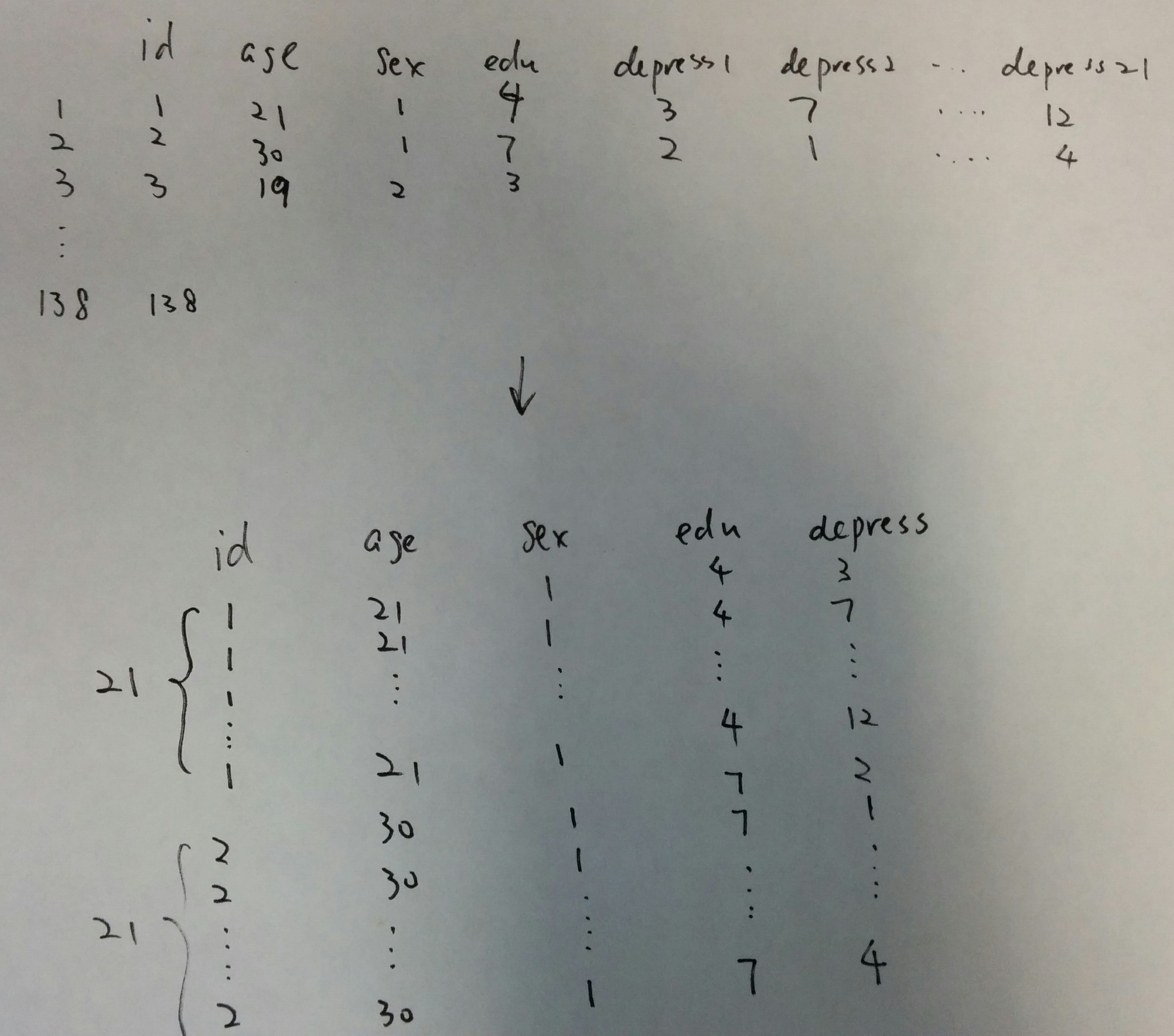
We now want to stack the depression item data together to get a long format data set as shown at the bottom of the above figure.
baseline.long <- baseline %>%
                  select(id, age, sex, edulevel,
                         starts_with('depress')) %>%
                  gather(starts_with('depress'),
                         key='item', value='depression') %>%
                  arrange(id)
baseline.long
## # A tibble: 2,898 x 6
##       id   age   sex edulevel item      depression
##    <dbl> <dbl> <dbl>    <dbl> <chr>          <dbl>
##  1     1    39     1        6 depress1           0
##  2     1    39     1        6 depress2           2
##  3     1    39     1        6 depress3           1
##  4     1    39     1        6 depress4           0
##  5     1    39     1        6 depress5           0
##  6     1    39     1        6 depress6           0
##  7     1    39     1        6 depress7           0
##  8     1    39     1        6 depress8           0
##  9     1    39     1        6 depress9           0
## 10     1    39     1        6 depress10          0
## # ... with 2,888 more rows- To organize the data, we used the function
gather(). The function takes multiple columns and collapses into key-value pairs, duplicating all other columns as needed. - To use the function, we need the following information
- The columns to be stacked.
key, the new column created to identify the data in the original data set.value, the new column created to save the information from the multiple columns.
3.6.2 From long format to wide format
Similarly, there are times to convert the long format data to wide format data. To do so, we use the spread() function.
baseline.wide <- baseline.long %>%
  spread(key=item, value=depression)

baseline.wide
## # A tibble: 138 x 25
##       id   age   sex edulevel depress1 depress10 depress11 depress12 depress13
##    <dbl> <dbl> <dbl>    <dbl>    <dbl>     <dbl>     <dbl>     <dbl>     <dbl>
##  1     1    39     1        6        0         0         1         3         0
##  2    27    18     2        2        0         1         0         0         0
##  3    28    18     2        4        1         1         1         1         1
##  4    31    18     2        2        0         1         0         0         0
##  5    32    18     2        2        1         5         0         1         1
##  6    34    21     2        3        1         0         1         0         0
##  7    35    21     1        3        0         0         0         0         1
##  8    36    23     1        3        0         0         0         0         0
##  9    37    20     2        3        1         1         0         0         3
## 10    38    20     2        3        0         0         0         0         0
## # ... with 128 more rows, and 16 more variables: depress14 <dbl>,
## #   depress15 <dbl>, depress16 <dbl>, depress17 <dbl>, depress18 <dbl>,
## #   depress19 <dbl>, depress2 <dbl>, depress20 <dbl>, depress21 <dbl>,
## #   depress3 <dbl>, depress4 <dbl>, depress5 <dbl>, depress6 <dbl>,
## #   depress7 <dbl>, depress8 <dbl>, depress9 <dbl>
3.6.2.1 Practice
Change the wide format data from parent1 to parent30 to long format.
Once finishing it, change it back to wide format
3.6.3 Unite and separate data
Sometimes, it might be useful to unite data together. For example,
baseline.unite <- baseline.wide %>%
  unite(col = depression, starts_with('depress'), sep=',')

baseline.unite
## # A tibble: 138 x 5
##       id   age   sex edulevel depression
##    <dbl> <dbl> <dbl>    <dbl> <chr>
##  1     1    39     1        6 0,0,1,3,0,1,2,1,2,1,2,2,3,0,1,0,0,0,0,0,0
##  2    27    18     2        2 0,1,0,0,0,0,1,1,0,0,0,1,1,0,0,0,0,0,0,1,0
##  3    28    18     2        4 1,1,1,1,1,1,1,1,1,0,1,1,1,0,1,0,1,1,2,1,1
##  4    31    18     2        2 0,1,0,0,0,0,0,1,0,0,0,0,1,0,0,0,0,0,0,0,0
##  5    32    18     2        2 1,5,0,1,1,0,2,0,0,1,3,0,0,1,1,1,2,0,0,2,0
##  6    34    21     2        3 1,0,1,0,0,2,0,0,0,0,0,1,0,0,0,0,2,0,0,1,0
##  7    35    21     1        3 0,0,0,0,1,0,0,0,0,1,0,0,0,0,1,0,1,0,0,0,0
##  8    36    23     1        3 0,0,0,0,0,0,0,0,0,1,1,0,0,0,1,0,0,0,0,1,0
##  9    37    20     2        3 1,1,0,0,3,0,1,0,1,0,0,0,1,0,1,0,0,0,1,1,1
## 10    38    20     2        3 0,0,0,0,0,0,0,0,0,0,0,0,1,0,0,0,0,0,0,0,0
## # ... with 128 more rows- The function
unite()is used here.colprovides the name of the new variable.sep, the symbol to connect the values.
We can also separate one variable to multiple variables using the function separate().
baseline.unite %>%
  separate(depression,
           into = paste0('depress', 1:21), sep=',',
           convert=TRUE)
## # A tibble: 138 x 25
##       id   age   sex edulevel depress1 depress2 depress3 depress4 depress5
##    <dbl> <dbl> <dbl>    <dbl>    <int>    <int>    <int>    <int>    <int>
##  1     1    39     1        6        0        0        1        3        0
##  2    27    18     2        2        0        1        0        0        0
##  3    28    18     2        4        1        1        1        1        1
##  4    31    18     2        2        0        1        0        0        0
##  5    32    18     2        2        1        5        0        1        1
##  6    34    21     2        3        1        0        1        0        0
##  7    35    21     1        3        0        0        0        0        1
##  8    36    23     1        3        0        0        0        0        0
##  9    37    20     2        3        1        1        0        0        3
## 10    38    20     2        3        0        0        0        0        0
## # ... with 128 more rows, and 16 more variables: depress6 <int>,
## #   depress7 <int>, depress8 <int>, depress9 <int>, depress10 <int>,
## #   depress11 <int>, depress12 <int>, depress13 <int>, depress14 <int>,
## #   depress15 <int>, depress16 <int>, depress17 <int>, depress18 <int>,
## # depress19 <int>, depress20 <int>, depress21 <int>- Fixed-width data
baseline.wide %>%
  select(id, age, sex, edulevel, paste0('depress', 1:21)) %>%
  na.omit() %>%
  unite(col = depression, starts_with('depress'), sep='') %>%
  mutate(temp = unlist(lapply(strsplit(depression, split=''), paste0, collapse=','))) %>%
  separate(temp, into = paste0('depress', 1:21), sep=',')
## # A tibble: 136 x 26
##       id   age   sex edulevel depression depress1 depress2 depress3 depress4
##    <dbl> <dbl> <dbl>    <dbl> <chr>      <chr>    <chr>    <chr>    <chr>
##  1     1    39     1        6 021000000~ 0        2        1        0
##  2    27    18     2        2 010000010~ 0        1        0        0
##  3    28    18     2        4 111011211~ 1        1        1        0
##  4    31    18     2        2 000000000~ 0        0        0        0
##  5    32    18     2        2 101120020~ 1        0        1        1
##  6    34    21     2        3 110020010~ 1        1        0        0
##  7    35    21     1        3 001010000~ 0        0        1        0
##  8    36    23     1        3 001000010~ 0        0        1        0
##  9    37    20     2        3 101000111~ 1        0        1        0
## 10    38    20     2        3 000000000~ 0        0        0        0
## # ... with 126 more rows, and 17 more variables: depress5 <chr>,
## #   depress6 <chr>, depress7 <chr>, depress8 <chr>, depress9 <chr>,
## #   depress10 <chr>, depress11 <chr>, depress12 <chr>, depress13 <chr>,
## #   depress14 <chr>, depress15 <chr>, depress16 <chr>, depress17 <chr>,
## #   depress18 <chr>, depress19 <chr>, depress20 <chr>, depress21 <chr>
3.7 Working with multiple data sets
3.7.1 Two data sets with the same variables but different participants
Consider the two data sets below. Each data set contains five participants with three variables.
dset1 <- tibble(id = 1:5,
                sex = c('m','m','f','f','f'),
                edu = sample(1:15, 5))
dset1
## # A tibble: 5 x 3
##      id sex     edu
##   <int> <chr> <int>
## 1     1 m         1
## 2     2 m        15
## 3     3 f         7
## 4     4 f        11
## 5     5 f         2

dset2 <- tibble(id = 6:10,
                sex = c('m','m','f','f','f'),
                edu = sample(1:15, 5))
dset2
## # A tibble: 5 x 3
##      id sex     edu
##   <int> <chr> <int>
## 1     6 m        10
## 2     7 m         3
## 3     8 f        15
## 4     9 f         6
## 5    10 f         7
We can use bind_rows from the package dplyr or rbind from R base.
bind_rows(dset1, dset2)
## # A tibble: 10 x 3
##       id sex     edu
##    <int> <chr> <int>
##  1     1 m         1
##  2     2 m        15
##  3     3 f         7
##  4     4 f        11
##  5     5 f         2
##  6     6 m        10
##  7     7 m         3
##  8     8 f        15
##  9     9 f         6
## 10    10 f         7
dset1 %>% bind_rows(dset2)
## # A tibble: 10 x 3
##       id sex     edu
##    <int> <chr> <int>
##  1     1 m         1
##  2     2 m        15
##  3     3 f         7
##  4     4 f        11
##  5     5 f         2
##  6     6 m        10
##  7     7 m         3
##  8     8 f        15
##  9     9 f         6
## 10    10 f         7

rbind(dset1, dset2)
## # A tibble: 10 x 3
##       id sex     edu
##    <int> <chr> <int>
##  1     1 m         1
##  2     2 m        15
##  3     3 f         7
##  4     4 f        11
##  5     5 f         2
##  6     6 m        10
##  7     7 m         3
##  8     8 f        15
##  9     9 f         6
## 10 10 f 7full_join(dset1, dset2)
## # A tibble: 10 x 3
## id sex edu
## <int> <chr> <int>
## 1 1 m 1
## 2 2 m 15
## 3 3 f 7
## 4 4 f 11
## 5 5 f 2
## 6 6 m 10
## 7 7 m 3
## 8 8 f 15
## 9 9 f 6
## 10 10 f 73.7.2 Two data sets with the same participants but different variables
dset1 <- tibble(id = 1:5,
                sex = c('m','m','f','f','f'),
                edu = sample(1:15, 5))
dset1
## # A tibble: 5 x 3
##      id sex     edu
##   <int> <chr> <int>
## 1     1 m         9
## 2     2 m        11
## 3     3 f         5
## 4     4 f        10
## 5     5 f        13

dset2 <- tibble(id = 1:5,
                math = round(rnorm(5),2),
                proportion = round(runif(5),2) )
dset2
## # A tibble: 5 x 3
##      id  math proportion
##   <int> <dbl>      <dbl>
## 1     1  2.16       0.55
## 2     2  1.95       0.66
## 3     3 -0.04       0.47
## 4     4 -0.56       0.4
## 5     5 -0.76       0.27
The function bind_cols or cbind can be used here. Notice the different treatment to the common variable id.
bind_cols(dset1, dset2)
## # A tibble: 5 x 6
##      id sex     edu   id1  math proportion
##   <int> <chr> <int> <int> <dbl>      <dbl>
## 1     1 m         9     1  2.16       0.55
## 2     2 m        11     2  1.95       0.66
## 3     3 f         5     3 -0.04       0.47
## 4     4 f        10     4 -0.56       0.4
## 5     5 f        13     5 -0.76       0.27

cbind(dset1, dset2)
##   id sex edu id  math proportion
## 1  1   m   9  1  2.16       0.55
## 2  2   m  11  2  1.95       0.66
## 3  3   f   5  3 -0.04       0.47
## 4  4   f  10  4 -0.56       0.40
## 5 5 f 13 5 -0.76 0.27full_join(dset1, dset2)
## # A tibble: 5 x 5
## id sex edu math proportion
## <int> <chr> <int> <dbl> <dbl>
## 1 1 m 9 2.16 0.55
## 2 2 m 11 1.95 0.66
## 3 3 f 5 -0.04 0.47
## 4 4 f 10 -0.56 0.4
## 5 5 f 13 -0.76 0.27Another function full_join can be useful here. It automatically matches the common variable in the two data sets.
3.7.3 Two data sets with partial same participants and variables
Consider the two data set below.
dset1 <- tibble(id = 1:5,
                sex = c('m','m','f','f','f'),
                edu = sample(1:15, 5))
dset1
## # A tibble: 5 x 3
##      id sex     edu
##   <int> <chr> <int>
## 1     1 m        14
## 2     2 m        12
## 3     3 f        15
## 4     4 f         4
## 5     5 f        11

dset2 <- tibble(id = 3:7,
                sex = c('f','f','f','m','m'),
                math = round(rnorm(5),2),
                proportion = round(runif(5),2) )
dset2
## # A tibble: 5 x 4
##      id sex    math proportion
##   <int> <chr> <dbl>      <dbl>
## 1     3 f      0.11      0.41
## 2     4 f      0.64      0.580
## 3     5 f      0.84      0.87
## 4     6 m     -0.03      0.41
## 5     7 m     -0.76      0.8
3.7.3.1 Combine all possible information based on a key variable, id here.
full_join(dset1, dset2)
## # A tibble: 7 x 5
##      id sex     edu   math proportion
##   <int> <chr> <int>  <dbl>      <dbl>
## 1     1 m        14  NA        NA
## 2     2 m        12  NA        NA
## 3     3 f        15   0.11      0.41
## 4     4 f         4   0.64      0.580
## 5     5 f        11   0.84      0.87
## 6     6 m        NA  -0.03      0.41
## 7     7 m        NA  -0.76      0.8

full_join(dset1, dset2, by='id')
## # A tibble: 7 x 6
##      id sex.x   edu sex.y   math proportion
##   <int> <chr> <int> <chr>  <dbl>      <dbl>
## 1     1 m        14 <NA>   NA        NA
## 2     2 m        12 <NA>   NA        NA
## 3     3 f        15 f       0.11      0.41
## 4     4 f         4 f       0.64      0.580
## 5     5 f        11 f       0.84      0.87
## 6     6 <NA>     NA m      -0.03      0.41
## 7     7 <NA>     NA m      -0.76      0.8
3.7.3.2 Keep all information in the first data set and add the matched information from the second data set
left_join(dset1, dset2)
## # A tibble: 5 x 5
##      id sex     edu  math proportion
##   <int> <chr> <int> <dbl>      <dbl>
## 1     1 m        14 NA        NA
## 2     2 m        12 NA        NA
## 3     3 f        15  0.11      0.41
## 4     4 f         4  0.64      0.580
## 5     5 f        11  0.84      0.87
3.7.3.3 Keep all information in the second data set and add the matched information from the first data set
right_join(dset1, dset2)
## # A tibble: 5 x 5
##      id sex     edu  math proportion
##   <int> <chr> <int> <dbl>      <dbl>
## 1     3 f        15  0.11      0.41
## 2     4 f         4  0.64      0.580
## 3     5 f        11  0.84      0.87
## 4     6 m        NA -0.03      0.41
## 5     7 m        NA -0.76      0.8
3.7.3.4 Keep the common information only
inner_join(dset1, dset2)
## # A tibble: 3 x 5
##      id sex     edu  math proportion
##   <int> <chr> <int> <dbl>      <dbl>
## 1     3 f        15  0.11      0.41
## 2     4 f         4  0.64      0.580
## 3     5 f        11  0.84      0.87
3.7.3.5 Remove the common information
anti_join(dset1, dset2)
## # A tibble: 2 x 3
##      id sex     edu
##   <int> <chr> <int>
## 1     1 m        14
## 2     2 m        12
From the help document.
inner_join(): return all rows from x where there are matching values in y, and all columns from x and y. If there are multiple matches between x and y, all combination of the matches are returned.left_join(): return all rows from x, and all columns from x and y. Rows in x with no match in y will have NA values in the new columns. If there are multiple matches between x and y, all combinations of the matches are returned.right_join(): return all rows from y, and all columns from x and y. Rows in y with no match in x will have NA values in the new columns. If there are multiple matches between x and y, all combinations of the matches are returned.full_join(): return all rows and all columns from both x and y. Where there are not matching values, returns NA for the one missing.anti_join(): return all rows from x where there are not matching values in y, keeping just columns from x.
3.7.4 When the key variable is not unique.
Suppose we want to recode the sex variable.
dset3 <- tibble(sex = c('m', 'f'), value = c(0, 1))To add the value of m and f to the first data set, we use
left_join(dset1, dset3)
## # A tibble: 5 x 4
##      id sex     edu value
##   <int> <chr> <int> <dbl>
## 1     1 m        14     0
## 2     2 m        12     0
## 3     3 f        15     1
## 4     4 f         4     1
## 5     5 f        11     1
3.8 Homework
The data file relig-daily.csv includes the daily data from the religious study. With the data, do the following.
- Read the data into R.
- In the data, “id” is the unique id of each participant and “survey” is the survey number (for example, at day 1, the survey number 1, at day 2, the survey number is 2, and so on).
- How many participants are there in the data sets?
- Obtain the total number of surveys for each participants
- relmin1 - relmin16, the number of minutes spent on different kinds of religious activities.
- Create a new variable to represent the total number of minutes spent on all religious activities for each survey and participant
- Calculate the average number of minutes across surveys of each participant
- Compare the average number of minutes spent on all religious activities between male and female participants
- Calculate the correlation between age and the average number of minutes spent on all religious activities